**16-825 : Neural Surfaces**
Student name: Abhishek Pavani
(#) 1. Sphere Tracing
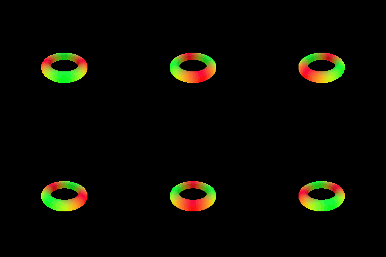
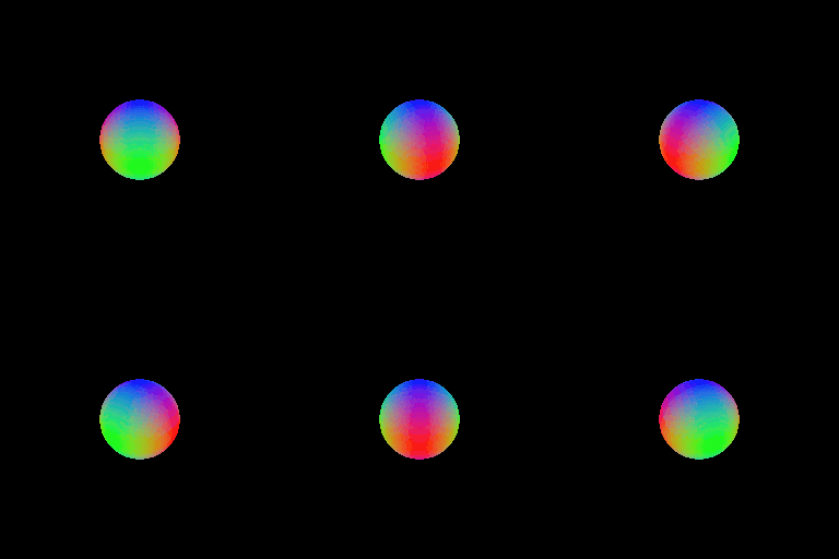
Sphere tracing is a technique used to trace the path of a ray as it travels through a 3D scene, using a signed distance function to determine the distance to the closest object.
The algorithmic details are mentioned below:
1. We start by choosing a starting point in 3D space and a direction for the ray. In our case we can choose the starting point as `origins`
2. We then evaluate the signed distance function at origin to determine the distance to the closest object in the scene.
3. We then move the starting point along the ray by the distance computed in step 2. Here the idea is that if we move by a distance equal to the signed distance, then we will reach the surfaces but never cross it. Even if we do, the sign of the signed distance will cause the point to be pushed on to the surface
4. Repeat steps 2 and 3 until the ray intersects an object or we reach the end of our max iterations.
5. Finally we set the mask to 1 where sdf < threshold.
Code Implementation:
```
while max_iters:
sdf_value = implicit_fn(points)
z_val += sdf_value.view(-1)
points = origins + z_val.unsqueeze(1) * directions
mask[sdf_value < eps_threshold] = 1
max_iters-=1
```
(##) Output
(#) 2. Optimizing a Neural SDF
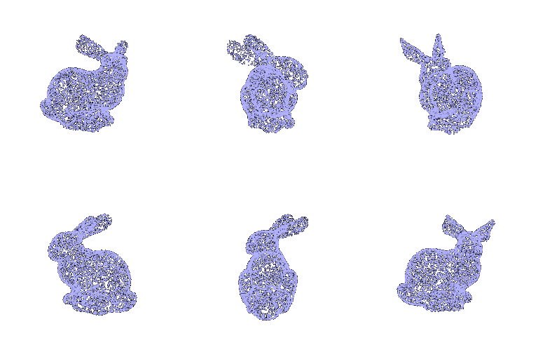
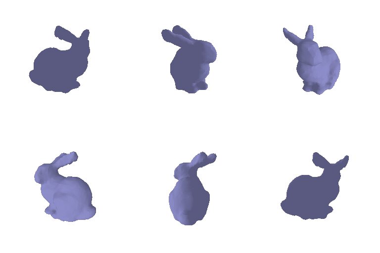
In this part, I implemented an MLP architecture for a neural SDF, and trained this neural SDF on point cloud data.
I did this by training the network to output aslack zero value at the observed points. To encourage the network to learn an SDF instead of an arbitrary function, I used a 'eikonal' regularization which enforces the gradients of the predictions to behave in a certain way. In particular, it is a property of the SDF to have norm of the gradients = 1
(##) Output
| Input | Optimized Neural SDF |
|-----------------------|-----------------------|
| ||
(##) Description of MLP and Eikonal loss
I defined an MLPwithInputSkips like I did in NeRF and then added an additional linear layer to output the per point SDF.
Eikonal loss is introduced to enforce the constraint that the norm of the gradient for an SDF should be 1. I used MSE Loss to force the gradients to converge to 1 after training.
` eikonal_loss = MSELoss(torch.linalg.norm(gradients,dim=-1),torch.ones_like(gradients))`
We additionally introduced point loss to ensure that the points lie on the surface. We enforce this by using MSELoss as shown below,
` point_loss = MSELoss(distances, 0)`
Config file I used are as follows:
```
implicit_function:
type: neural_surface
n_harmonic_functions_xyz: 4
n_layers_distance: 6
n_hidden_neurons_distance: 128
append_distance: []
n_layers_color: 2
n_hidden_neurons_color: 128
append_color: []
```
(##) Hyperparameter Tuning
| Eikonal weight (Weight Regularization) | Optimized Neural SDF |
|-----------------------|-----------------------|
| 0.005 ||
| 0.04 ||
| 0.07 ||
| 0.5 ||
(#) 3. VolSDF
In this part, I implemented a function to convert SDF -> volume density and extend the NeuralSurface class to predict color.
Color Prediction: I defined a color MLP with input skips, like I did for density in the previous step. I added another input layer in which the out channels were 3. I then pass the output from the linear layer to sigmoid activation to rescale the colors between 0 and 1.
SDF -> Density : I implemented the equation mentioned in the section 3.1 of the [VolSDF Paper](https://arxiv.org/pdf/2106.12052.pdf).
The formula for density depends on the signed distance function and is stated as follows
`sigma(x) = - alpha * psi_beta(-sdf)`
```
where psi_beta(s) = 0.5 * exp(sdf/beta) when sdf<=0
= 1 - 0.5 * exp(-sdf/beta) when sdf>0
```
(###) Alpha and beta parameters:
Alpha denotes the density of points. If a point is inside the surface the value is alpha and if it is outside the density is 0.
The transition of density from outside the surface to inside is controlled by the parameter beta.
In the paper both alpha and beta are learnable parameters but we have kept them to be constant in this implementation.
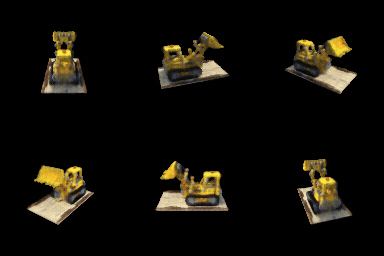
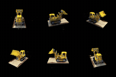
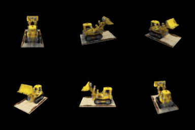
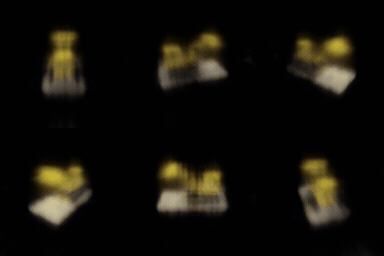
**1. How does high beta bias your learned SDF? What about low beta?**
A high value of beta intuitively tells us that the transition of density from inside the surface to outside the surface should be slow, meaning the volume appears to be too smooth or transparent.
Whereas a low beta on the other hand, would mean that the transition happens too quickly and the output looks sharper as opposed to being smoother.
This can be qualitatively seen the table below
**Would an SDF be easier to train with volume rendering and low beta or high beta? Why?**
When it comes to training with volume rendering, using low beta values in SDF
is more effective than high beta values. High beta values result in density that is
spread out over a larger area, making the object more transparent.
This is because the conversion from SDF to density becomes more similar across a wider range of values,
and in extreme cases can be constant across all values of SDF.
On the other hand, low beta values help to constrain density closer to the object's surface,
resulting in better modeling of the 3D object. This is because the density is higher near the surface(sdf=0) and quickly reaches 0 as you move away from the surface, making it easier for the model to learn useful SDF to represent the 3D object.
**3. Would you be more likely to learn an accurate surface with high beta or low beta? Why?**
As mentioned above, a low beta helps us capture the intricacies of the volume and is a more
accurate representation of the sdf. Mathematically, a low beta means a lower variance of the cdf and on the other hand a higher value of beta means higher variance and hence a smoothed/blurry output
| Beta values | Output Geometry | Output Color|
|-------------|-----------------|-------------|
| 0.0005 |||
| 0.005 |||
| 0.05 |||
| 0.5 |||
| 1 | No Geometry||
| 2 | No Geometry||
(#) 4. Phong Relighting
In this part, I implemented the Phong reflection model in order to render the SDF volume I trained under different lighting conditions.
|Phong(without color)|Phong (with color)|
|----|-----|
|||
(#) 5. Neural Surface Extras
(##) 5.1 Render a large scene with sphere tracing
(##) 5.2 Experiments with fewer training views(20 views)
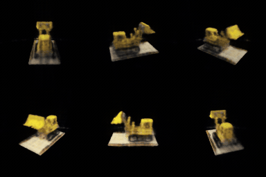
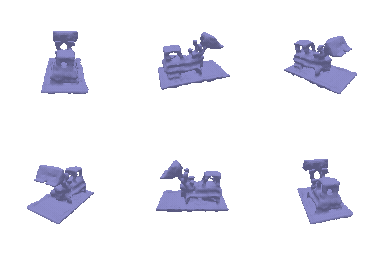
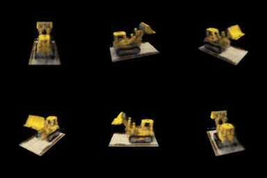
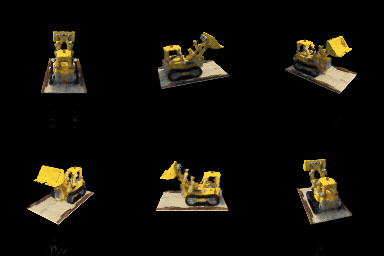
I tried experimenting with 1 view, 10 views and 20 views and have tabulated my results below.
As seen below VolSDF performs reasonably well even for 10 views whereas I got no output for 10 views in NeRF. NeRF starts showing some output at 50 views but it comes with artifacts.
|Views| VolSDF(geometry) | VolSDF (color) | NeRF |
|-----|-------------------|--------------------|------|
|1||||
|10||||
|20||||
|50||||
(##) 5.3 Neural Implicit Surface (NeUS)
I replaced the density estimation in the sdf to density estimation by the following equation
`density = s * exp(-sdf *s) / (1 + exp(-sdf * s))**2`
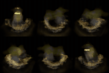
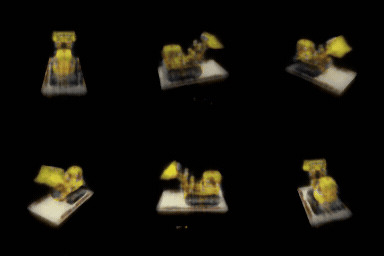
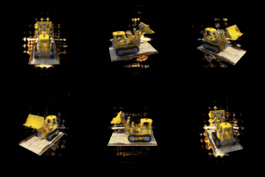
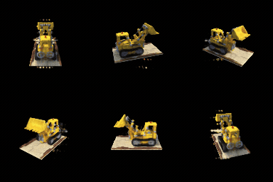
Here I tried different values of 's' to get the following outputs. Lower values of 's' tend to give a blobby output, whereas too high of an 's' value results in the loss going to nan and get no output.
For this particular lego sdf, a 's' value of 50 and 100 seem to have captured intricate details.
| s value | NeUS (Geometry) | Density Field|
|---------|-----------------|--------------|
|1|||
|10|||
|50|||
|100|||
 (#) 1. Sphere Tracing
Sphere tracing is a technique used to trace the path of a ray as it travels through a 3D scene, using a signed distance function to determine the distance to the closest object.
The algorithmic details are mentioned below:
1. We start by choosing a starting point in 3D space and a direction for the ray. In our case we can choose the starting point as `origins`
2. We then evaluate the signed distance function at origin to determine the distance to the closest object in the scene.
3. We then move the starting point along the ray by the distance computed in step 2. Here the idea is that if we move by a distance equal to the signed distance, then we will reach the surfaces but never cross it. Even if we do, the sign of the signed distance will cause the point to be pushed on to the surface
4. Repeat steps 2 and 3 until the ray intersects an object or we reach the end of our max iterations.
5. Finally we set the mask to 1 where sdf < threshold.
Code Implementation:
```
while max_iters:
sdf_value = implicit_fn(points)
z_val += sdf_value.view(-1)
points = origins + z_val.unsqueeze(1) * directions
mask[sdf_value < eps_threshold] = 1
max_iters-=1
```
(##) Output
(#) 1. Sphere Tracing
Sphere tracing is a technique used to trace the path of a ray as it travels through a 3D scene, using a signed distance function to determine the distance to the closest object.
The algorithmic details are mentioned below:
1. We start by choosing a starting point in 3D space and a direction for the ray. In our case we can choose the starting point as `origins`
2. We then evaluate the signed distance function at origin to determine the distance to the closest object in the scene.
3. We then move the starting point along the ray by the distance computed in step 2. Here the idea is that if we move by a distance equal to the signed distance, then we will reach the surfaces but never cross it. Even if we do, the sign of the signed distance will cause the point to be pushed on to the surface
4. Repeat steps 2 and 3 until the ray intersects an object or we reach the end of our max iterations.
5. Finally we set the mask to 1 where sdf < threshold.
Code Implementation:
```
while max_iters:
sdf_value = implicit_fn(points)
z_val += sdf_value.view(-1)
points = origins + z_val.unsqueeze(1) * directions
mask[sdf_value < eps_threshold] = 1
max_iters-=1
```
(##) Output
 (#) 2. Optimizing a Neural SDF
In this part, I implemented an MLP architecture for a neural SDF, and trained this neural SDF on point cloud data.
I did this by training the network to output aslack zero value at the observed points. To encourage the network to learn an SDF instead of an arbitrary function, I used a 'eikonal' regularization which enforces the gradients of the predictions to behave in a certain way. In particular, it is a property of the SDF to have norm of the gradients = 1
(##) Output
| Input | Optimized Neural SDF |
|-----------------------|-----------------------|
|
(#) 2. Optimizing a Neural SDF
In this part, I implemented an MLP architecture for a neural SDF, and trained this neural SDF on point cloud data.
I did this by training the network to output aslack zero value at the observed points. To encourage the network to learn an SDF instead of an arbitrary function, I used a 'eikonal' regularization which enforces the gradients of the predictions to behave in a certain way. In particular, it is a property of the SDF to have norm of the gradients = 1
(##) Output
| Input | Optimized Neural SDF |
|-----------------------|-----------------------|
| |
| |
(##) Description of MLP and Eikonal loss
I defined an MLPwithInputSkips like I did in NeRF and then added an additional linear layer to output the per point SDF.
Eikonal loss is introduced to enforce the constraint that the norm of the gradient for an SDF should be 1. I used MSE Loss to force the gradients to converge to 1 after training.
` eikonal_loss = MSELoss(torch.linalg.norm(gradients,dim=-1),torch.ones_like(gradients))`
We additionally introduced point loss to ensure that the points lie on the surface. We enforce this by using MSELoss as shown below,
` point_loss = MSELoss(distances, 0)`
Config file I used are as follows:
```
implicit_function:
type: neural_surface
n_harmonic_functions_xyz: 4
n_layers_distance: 6
n_hidden_neurons_distance: 128
append_distance: []
n_layers_color: 2
n_hidden_neurons_color: 128
append_color: []
```
(##) Hyperparameter Tuning
| Eikonal weight (Weight Regularization) | Optimized Neural SDF |
|-----------------------|-----------------------|
| 0.005 |
|
(##) Description of MLP and Eikonal loss
I defined an MLPwithInputSkips like I did in NeRF and then added an additional linear layer to output the per point SDF.
Eikonal loss is introduced to enforce the constraint that the norm of the gradient for an SDF should be 1. I used MSE Loss to force the gradients to converge to 1 after training.
` eikonal_loss = MSELoss(torch.linalg.norm(gradients,dim=-1),torch.ones_like(gradients))`
We additionally introduced point loss to ensure that the points lie on the surface. We enforce this by using MSELoss as shown below,
` point_loss = MSELoss(distances, 0)`
Config file I used are as follows:
```
implicit_function:
type: neural_surface
n_harmonic_functions_xyz: 4
n_layers_distance: 6
n_hidden_neurons_distance: 128
append_distance: []
n_layers_color: 2
n_hidden_neurons_color: 128
append_color: []
```
(##) Hyperparameter Tuning
| Eikonal weight (Weight Regularization) | Optimized Neural SDF |
|-----------------------|-----------------------|
| 0.005 |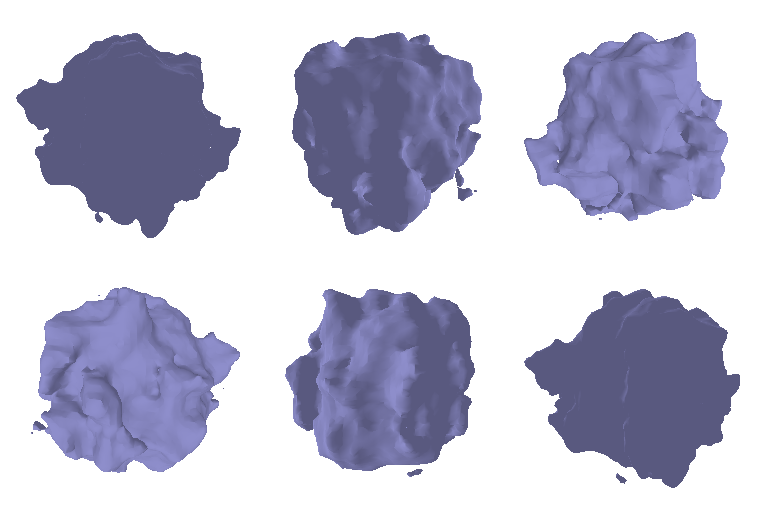 |
| 0.04 |
|
| 0.04 |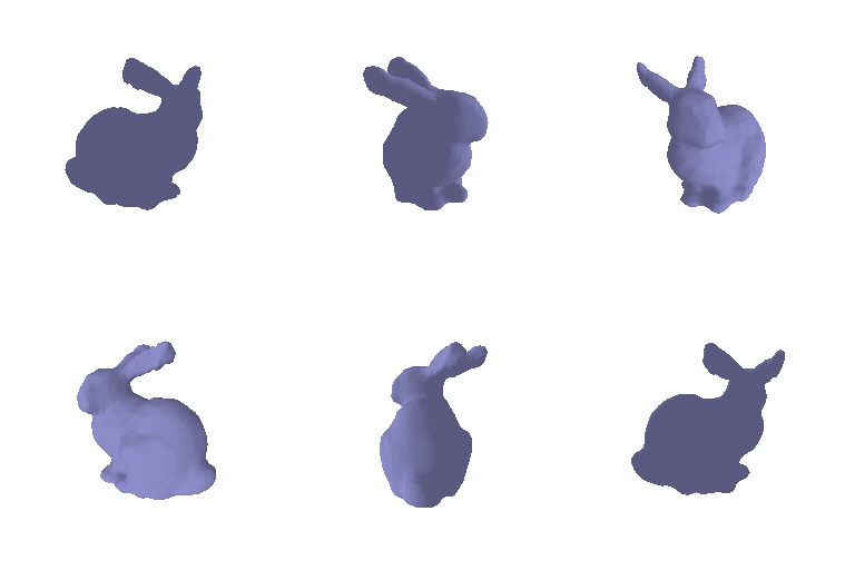 |
| 0.07 |
|
| 0.07 | |
| 0.5 |
|
| 0.5 | |
(#) 3. VolSDF
In this part, I implemented a function to convert SDF -> volume density and extend the NeuralSurface class to predict color.
Color Prediction: I defined a color MLP with input skips, like I did for density in the previous step. I added another input layer in which the out channels were 3. I then pass the output from the linear layer to sigmoid activation to rescale the colors between 0 and 1.
SDF -> Density : I implemented the equation mentioned in the section 3.1 of the [VolSDF Paper](https://arxiv.org/pdf/2106.12052.pdf).
The formula for density depends on the signed distance function and is stated as follows
`sigma(x) = - alpha * psi_beta(-sdf)`
```
where psi_beta(s) = 0.5 * exp(sdf/beta) when sdf<=0
= 1 - 0.5 * exp(-sdf/beta) when sdf>0
```
(###) Alpha and beta parameters:
Alpha denotes the density of points. If a point is inside the surface the value is alpha and if it is outside the density is 0.
The transition of density from outside the surface to inside is controlled by the parameter beta.
In the paper both alpha and beta are learnable parameters but we have kept them to be constant in this implementation.
**1. How does high beta bias your learned SDF? What about low beta?**
A high value of beta intuitively tells us that the transition of density from inside the surface to outside the surface should be slow, meaning the volume appears to be too smooth or transparent.
Whereas a low beta on the other hand, would mean that the transition happens too quickly and the output looks sharper as opposed to being smoother.
This can be qualitatively seen the table below
**Would an SDF be easier to train with volume rendering and low beta or high beta? Why?**
When it comes to training with volume rendering, using low beta values in SDF
is more effective than high beta values. High beta values result in density that is
spread out over a larger area, making the object more transparent.
This is because the conversion from SDF to density becomes more similar across a wider range of values,
and in extreme cases can be constant across all values of SDF.
On the other hand, low beta values help to constrain density closer to the object's surface,
resulting in better modeling of the 3D object. This is because the density is higher near the surface(sdf=0) and quickly reaches 0 as you move away from the surface, making it easier for the model to learn useful SDF to represent the 3D object.
**3. Would you be more likely to learn an accurate surface with high beta or low beta? Why?**
As mentioned above, a low beta helps us capture the intricacies of the volume and is a more
accurate representation of the sdf. Mathematically, a low beta means a lower variance of the cdf and on the other hand a higher value of beta means higher variance and hence a smoothed/blurry output
| Beta values | Output Geometry | Output Color|
|-------------|-----------------|-------------|
| 0.0005 |
|
(#) 3. VolSDF
In this part, I implemented a function to convert SDF -> volume density and extend the NeuralSurface class to predict color.
Color Prediction: I defined a color MLP with input skips, like I did for density in the previous step. I added another input layer in which the out channels were 3. I then pass the output from the linear layer to sigmoid activation to rescale the colors between 0 and 1.
SDF -> Density : I implemented the equation mentioned in the section 3.1 of the [VolSDF Paper](https://arxiv.org/pdf/2106.12052.pdf).
The formula for density depends on the signed distance function and is stated as follows
`sigma(x) = - alpha * psi_beta(-sdf)`
```
where psi_beta(s) = 0.5 * exp(sdf/beta) when sdf<=0
= 1 - 0.5 * exp(-sdf/beta) when sdf>0
```
(###) Alpha and beta parameters:
Alpha denotes the density of points. If a point is inside the surface the value is alpha and if it is outside the density is 0.
The transition of density from outside the surface to inside is controlled by the parameter beta.
In the paper both alpha and beta are learnable parameters but we have kept them to be constant in this implementation.
**1. How does high beta bias your learned SDF? What about low beta?**
A high value of beta intuitively tells us that the transition of density from inside the surface to outside the surface should be slow, meaning the volume appears to be too smooth or transparent.
Whereas a low beta on the other hand, would mean that the transition happens too quickly and the output looks sharper as opposed to being smoother.
This can be qualitatively seen the table below
**Would an SDF be easier to train with volume rendering and low beta or high beta? Why?**
When it comes to training with volume rendering, using low beta values in SDF
is more effective than high beta values. High beta values result in density that is
spread out over a larger area, making the object more transparent.
This is because the conversion from SDF to density becomes more similar across a wider range of values,
and in extreme cases can be constant across all values of SDF.
On the other hand, low beta values help to constrain density closer to the object's surface,
resulting in better modeling of the 3D object. This is because the density is higher near the surface(sdf=0) and quickly reaches 0 as you move away from the surface, making it easier for the model to learn useful SDF to represent the 3D object.
**3. Would you be more likely to learn an accurate surface with high beta or low beta? Why?**
As mentioned above, a low beta helps us capture the intricacies of the volume and is a more
accurate representation of the sdf. Mathematically, a low beta means a lower variance of the cdf and on the other hand a higher value of beta means higher variance and hence a smoothed/blurry output
| Beta values | Output Geometry | Output Color|
|-------------|-----------------|-------------|
| 0.0005 |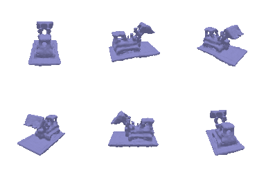 |
| |
| 0.005 |
|
| 0.005 |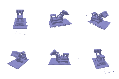 |
| |
| 0.05 |
|
| 0.05 |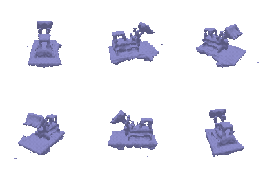 |
| |
| 0.5 |
|
| 0.5 |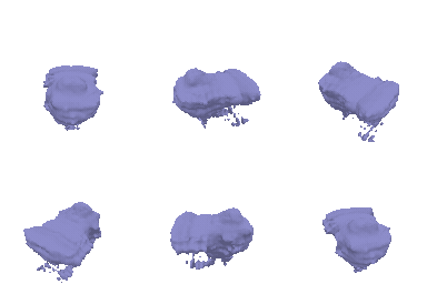 |
| |
| 1 | No Geometry|
|
| 1 | No Geometry| |
| 2 | No Geometry|
|
| 2 | No Geometry| |
(#) 4. Phong Relighting
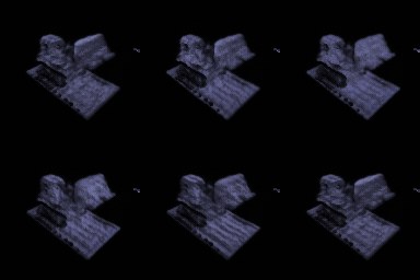
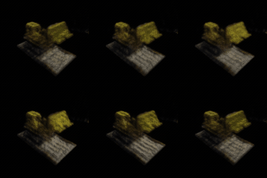
In this part, I implemented the Phong reflection model in order to render the SDF volume I trained under different lighting conditions.
|Phong(without color)|Phong (with color)|
|----|-----|
|
|
(#) 4. Phong Relighting
In this part, I implemented the Phong reflection model in order to render the SDF volume I trained under different lighting conditions.
|Phong(without color)|Phong (with color)|
|----|-----|
| |
| |
(#) 5. Neural Surface Extras
(##) 5.1 Render a large scene with sphere tracing
(##) 5.2 Experiments with fewer training views(20 views)
I tried experimenting with 1 view, 10 views and 20 views and have tabulated my results below.
As seen below VolSDF performs reasonably well even for 10 views whereas I got no output for 10 views in NeRF. NeRF starts showing some output at 50 views but it comes with artifacts.
|Views| VolSDF(geometry) | VolSDF (color) | NeRF |
|-----|-------------------|--------------------|------|
|1|
|
(#) 5. Neural Surface Extras
(##) 5.1 Render a large scene with sphere tracing
(##) 5.2 Experiments with fewer training views(20 views)
I tried experimenting with 1 view, 10 views and 20 views and have tabulated my results below.
As seen below VolSDF performs reasonably well even for 10 views whereas I got no output for 10 views in NeRF. NeRF starts showing some output at 50 views but it comes with artifacts.
|Views| VolSDF(geometry) | VolSDF (color) | NeRF |
|-----|-------------------|--------------------|------|
|1|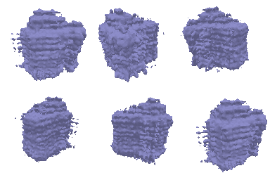 |
| |
| |
|10|
|
|10|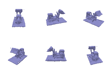 |
| |
| |
| |
| |
(##) 5.3 Neural Implicit Surface (NeUS)
I replaced the density estimation in the sdf to density estimation by the following equation
`density = s * exp(-sdf *s) / (1 + exp(-sdf * s))**2`
Here I tried different values of 's' to get the following outputs. Lower values of 's' tend to give a blobby output, whereas too high of an 's' value results in the loss going to nan and get no output.
For this particular lego sdf, a 's' value of 50 and 100 seem to have captured intricate details.
| s value | NeUS (Geometry) | Density Field|
|---------|-----------------|--------------|
|1|
|
(##) 5.3 Neural Implicit Surface (NeUS)
I replaced the density estimation in the sdf to density estimation by the following equation
`density = s * exp(-sdf *s) / (1 + exp(-sdf * s))**2`
Here I tried different values of 's' to get the following outputs. Lower values of 's' tend to give a blobby output, whereas too high of an 's' value results in the loss going to nan and get no output.
For this particular lego sdf, a 's' value of 50 and 100 seem to have captured intricate details.
| s value | NeUS (Geometry) | Density Field|
|---------|-----------------|--------------|
|1|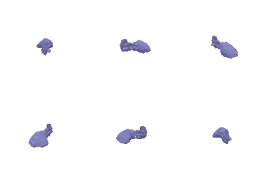 |
| |
|10|
|
|10|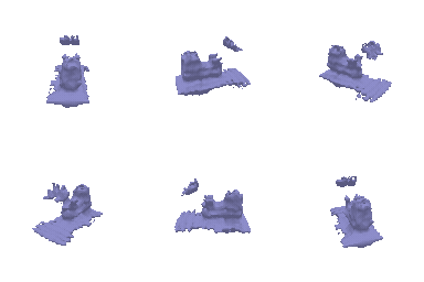 |
| |
|50|
|
|50|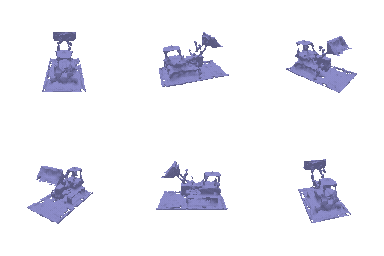 |
| |
|100|
|
|100|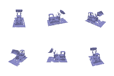 |
| |
|