**16-825 : Single View to 3D**
Student name: Abhishek Pavani
(#) 1. Exploring loss functions
This section will involve defining a loss function, for fitting voxels, point clouds and meshes.
(##) 1.1. Fitting a voxel grid
| Voxel Target | Voxel Optimized |
|-----------------------|------------------------|
| | |
| | |
| | |
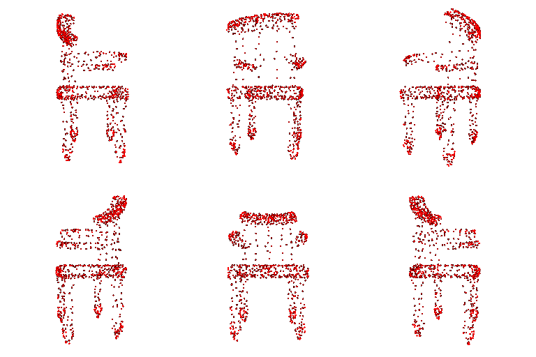
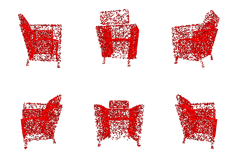
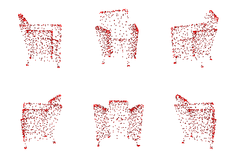
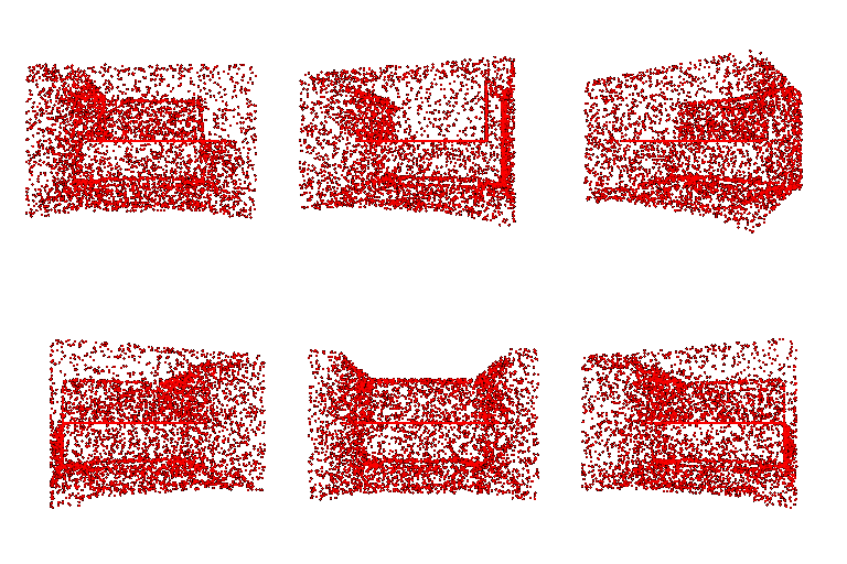
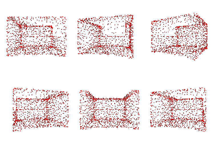
(##) 1.2. Fitting a point cloud
| Pointcloud Target | Pointcloud Optimized |
|-----------------------|------------------------|
| | |
| | |
| | |
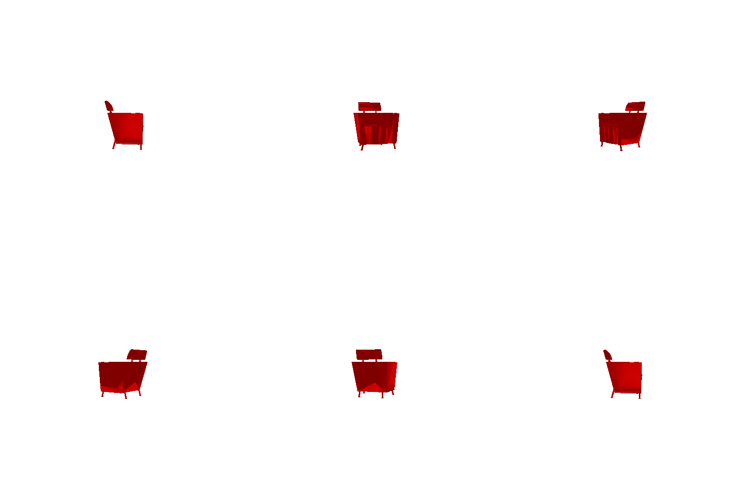
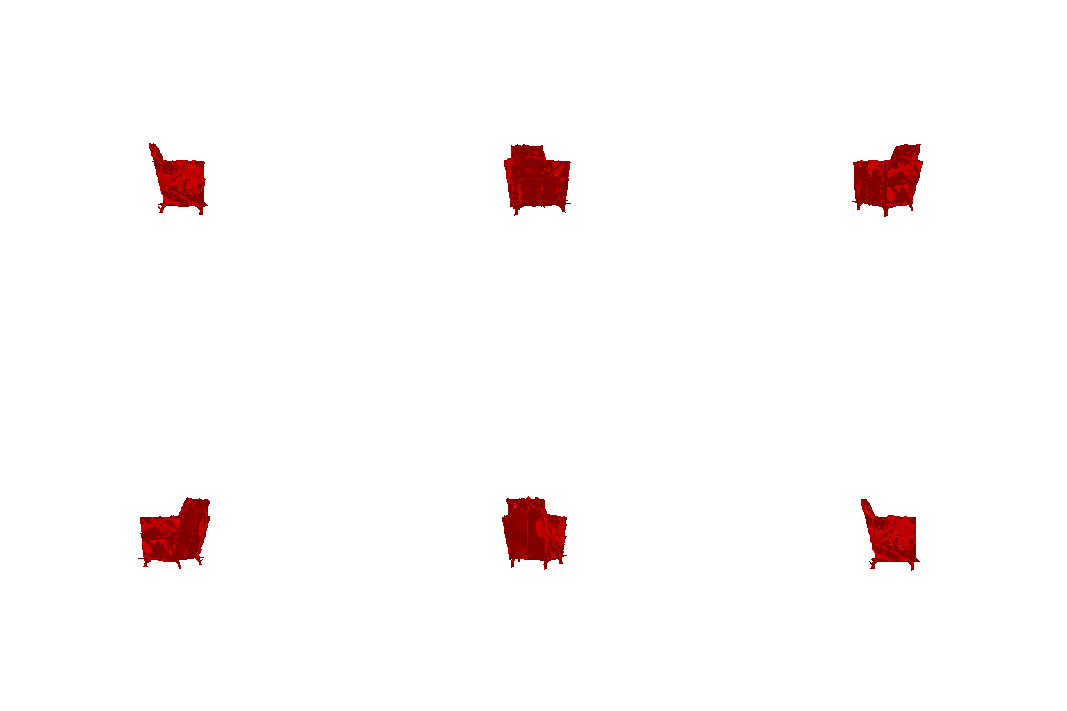
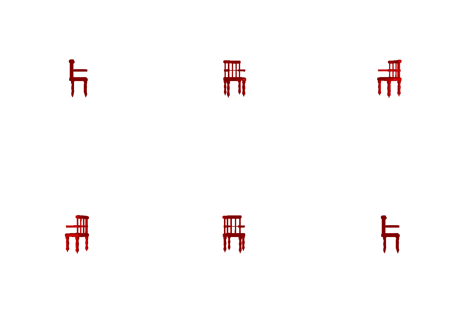
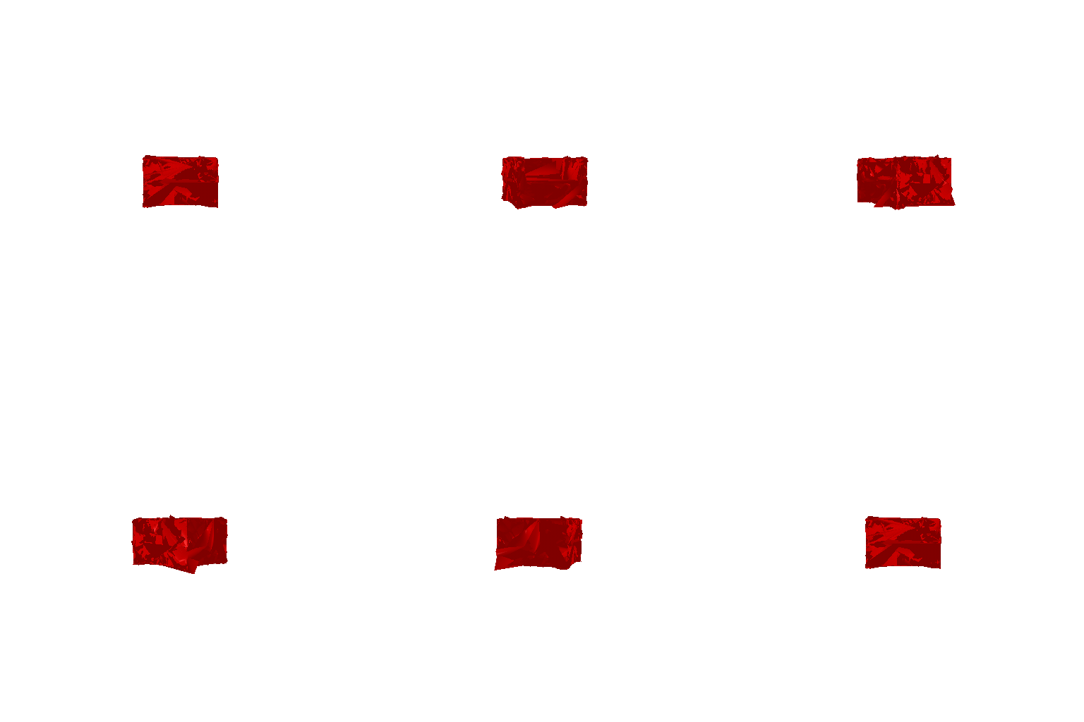
(##) 1.3. Fitting a mesh
| Mesh Target | Mesh Optimized |
|-----------------------|------------------------|
| | |
| | |
| | |
(#) 2. Practicing with Meshes
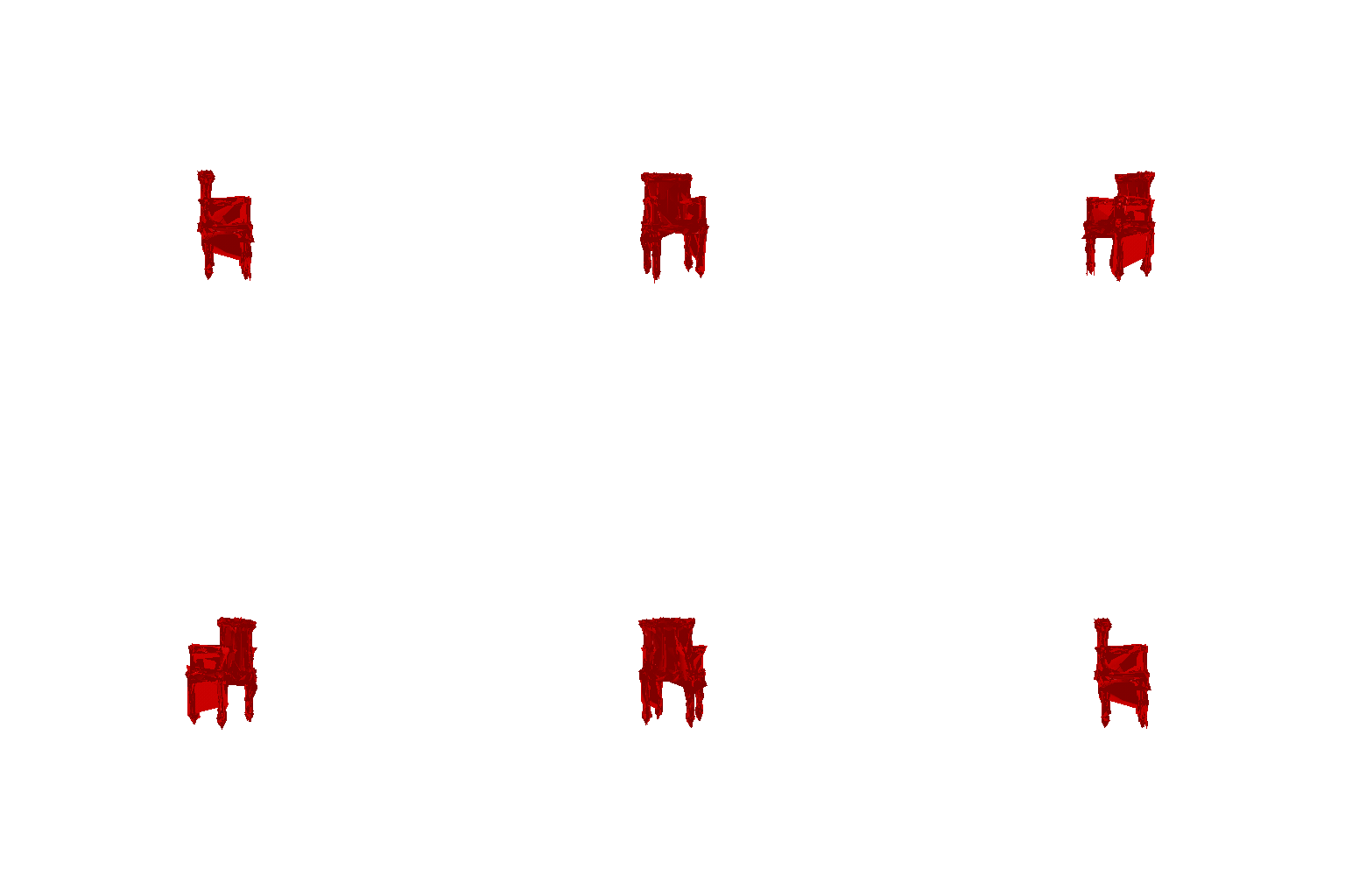
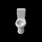
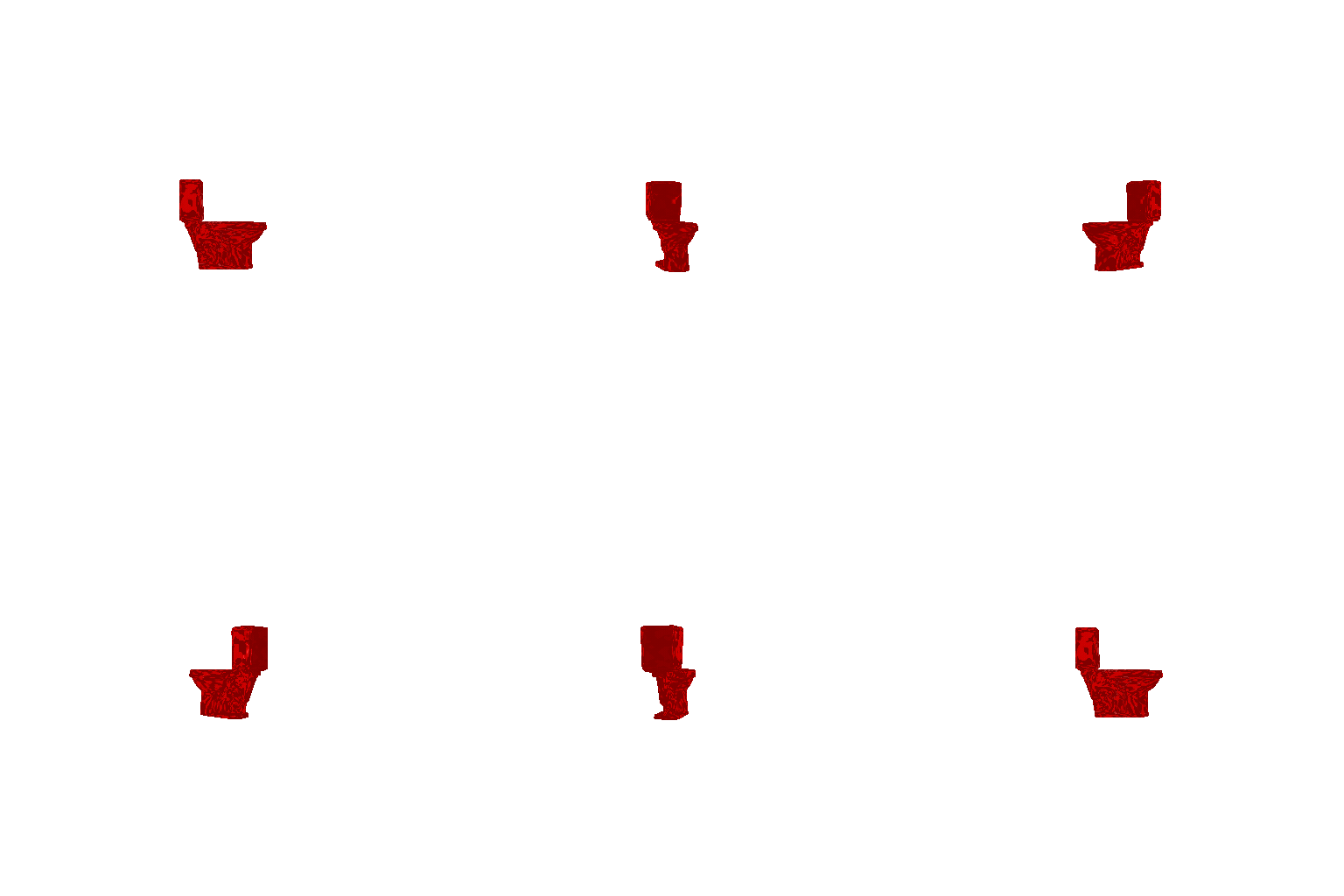
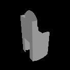
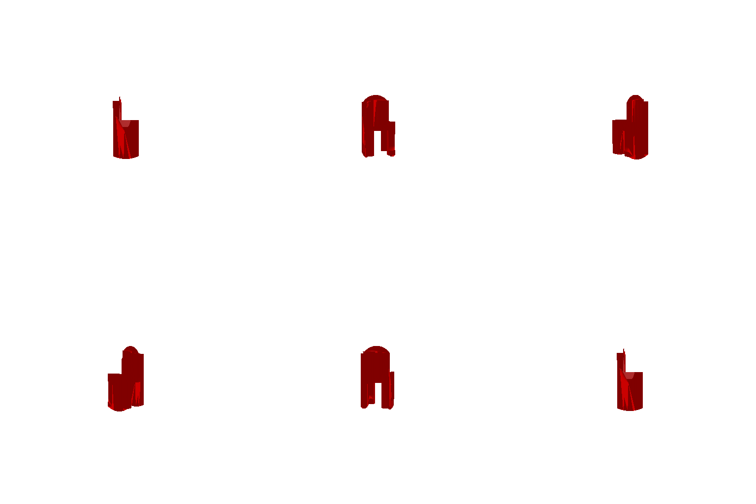
(##) 2.1 Image to voxel grid
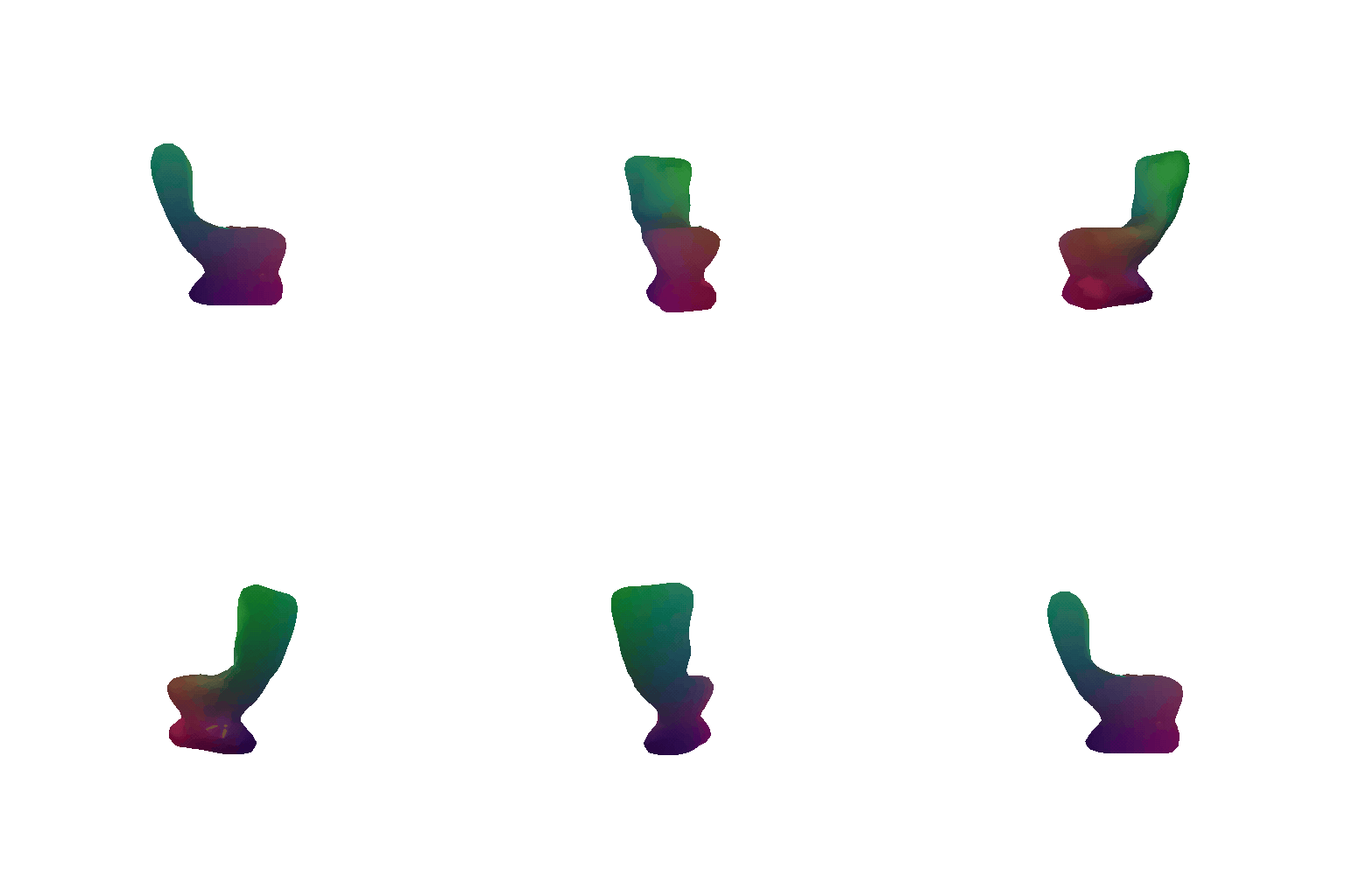
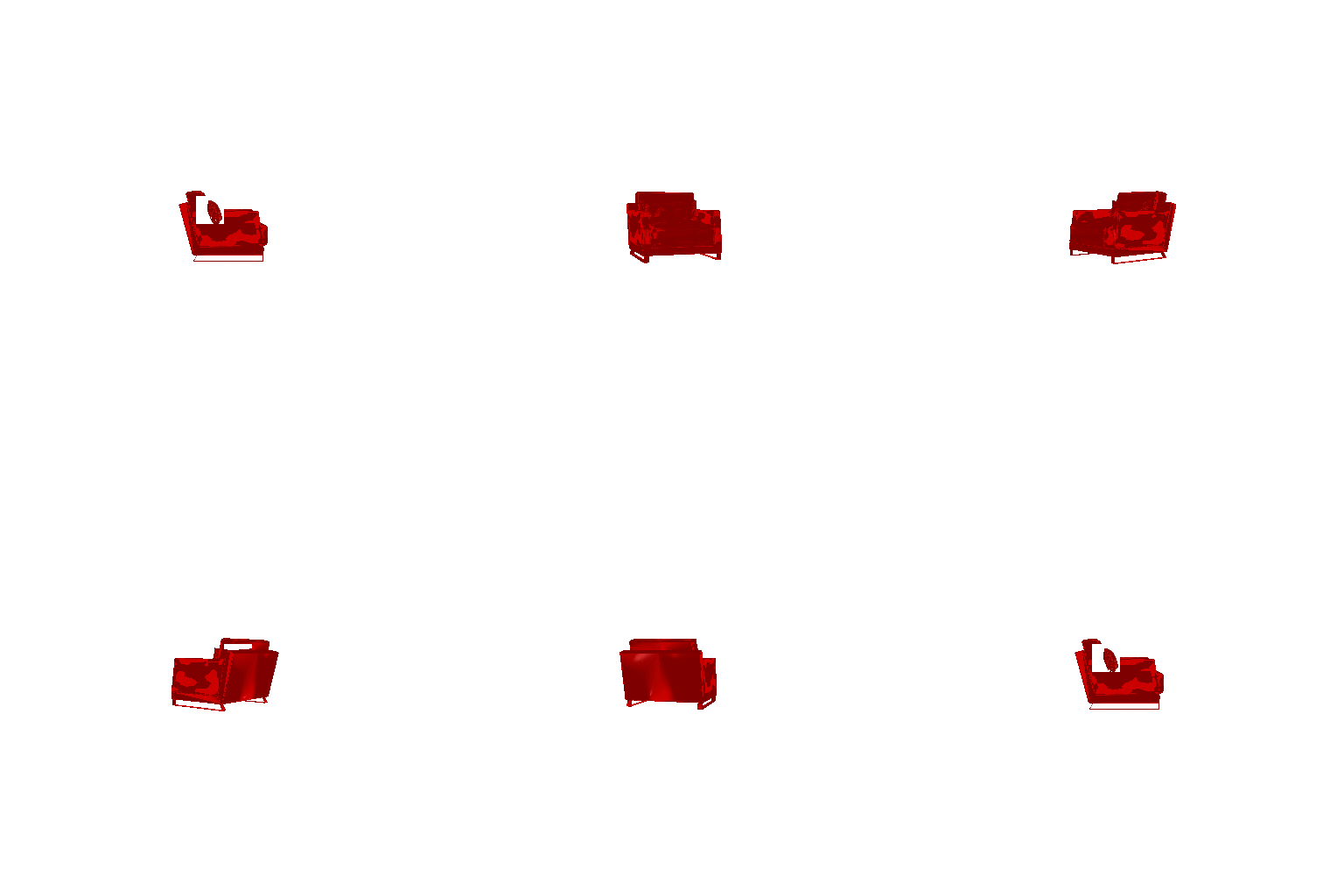
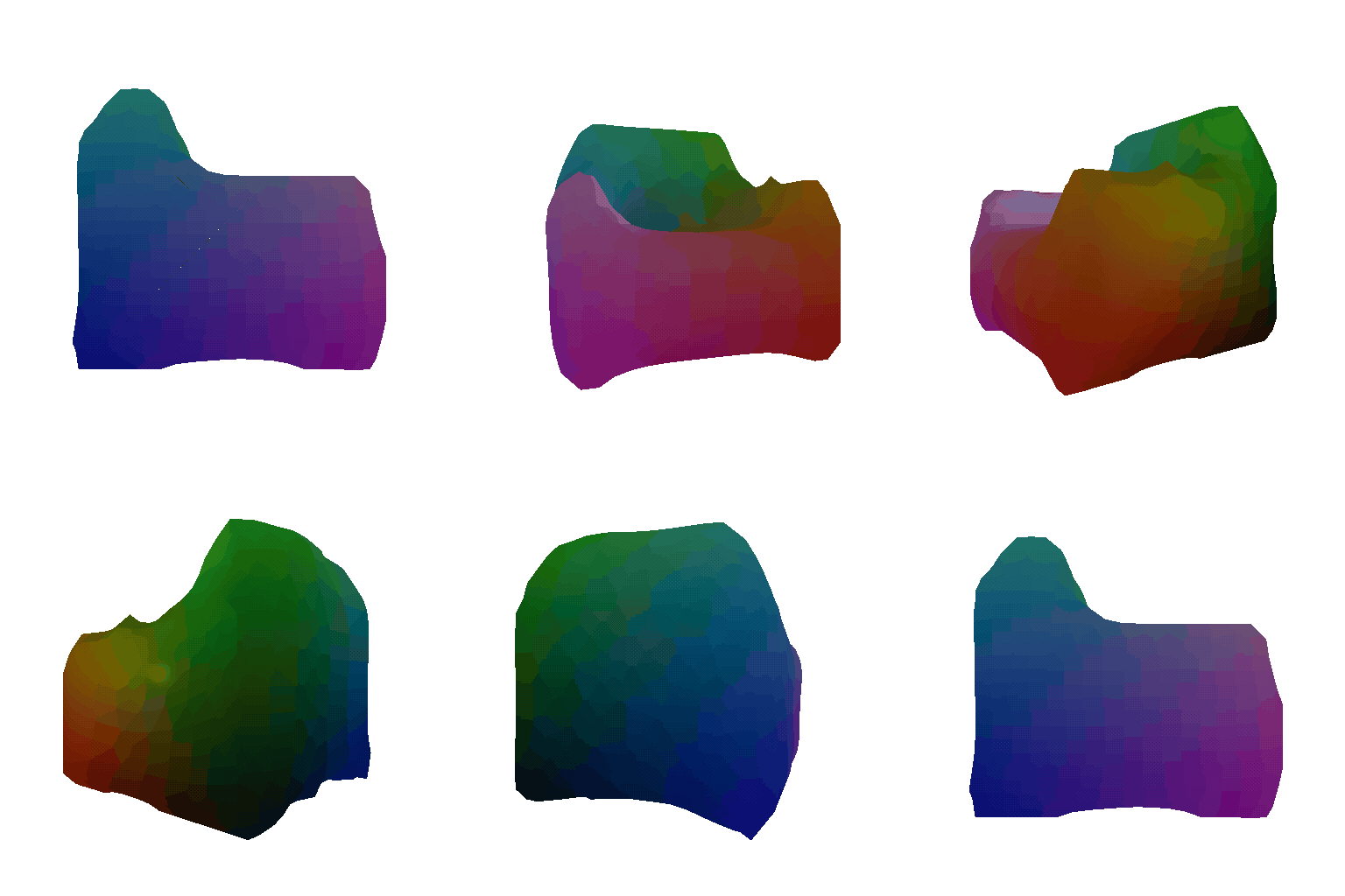
| Image | Ground truth Mesh | Prediction (Voxel) |
|-----------------------|------------------------|------------------------|
| | | |
| | | |
| | | |
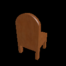
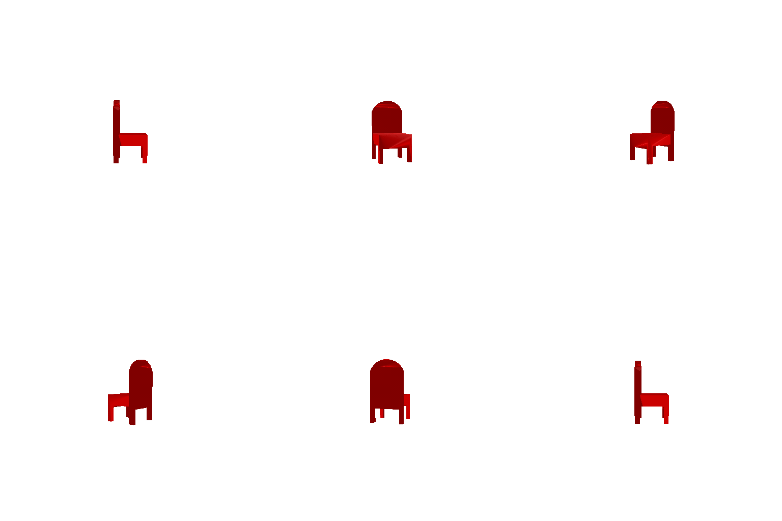
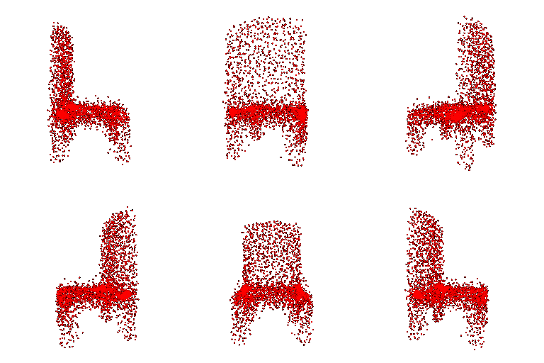
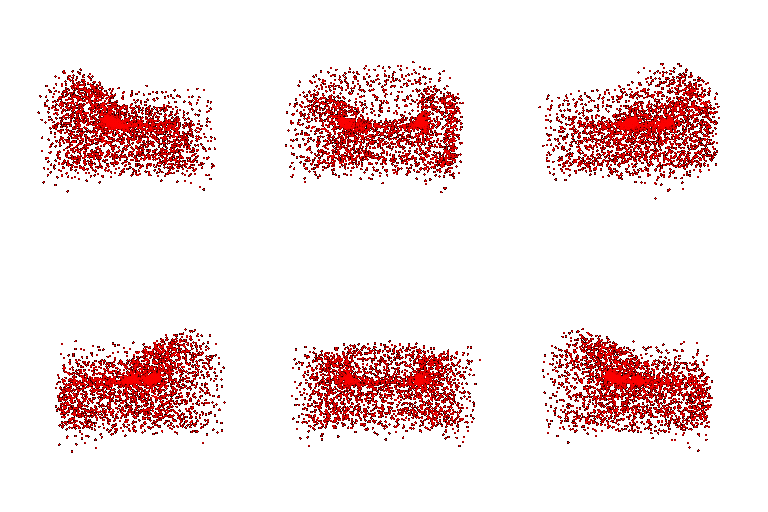
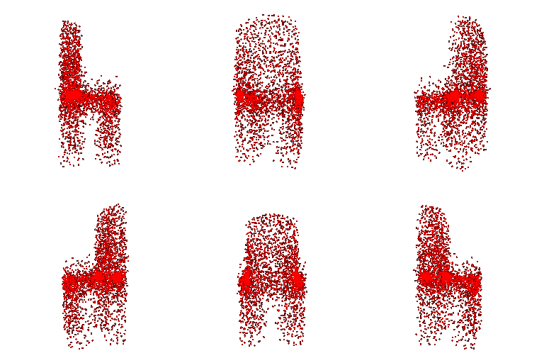
(##) 2.2 Image to point cloud
| Image | Ground truth Mesh | Prediction (Point cloud) |
|-----------------------|------------------------|------------------------|
| | | |
| | | |
| | | |
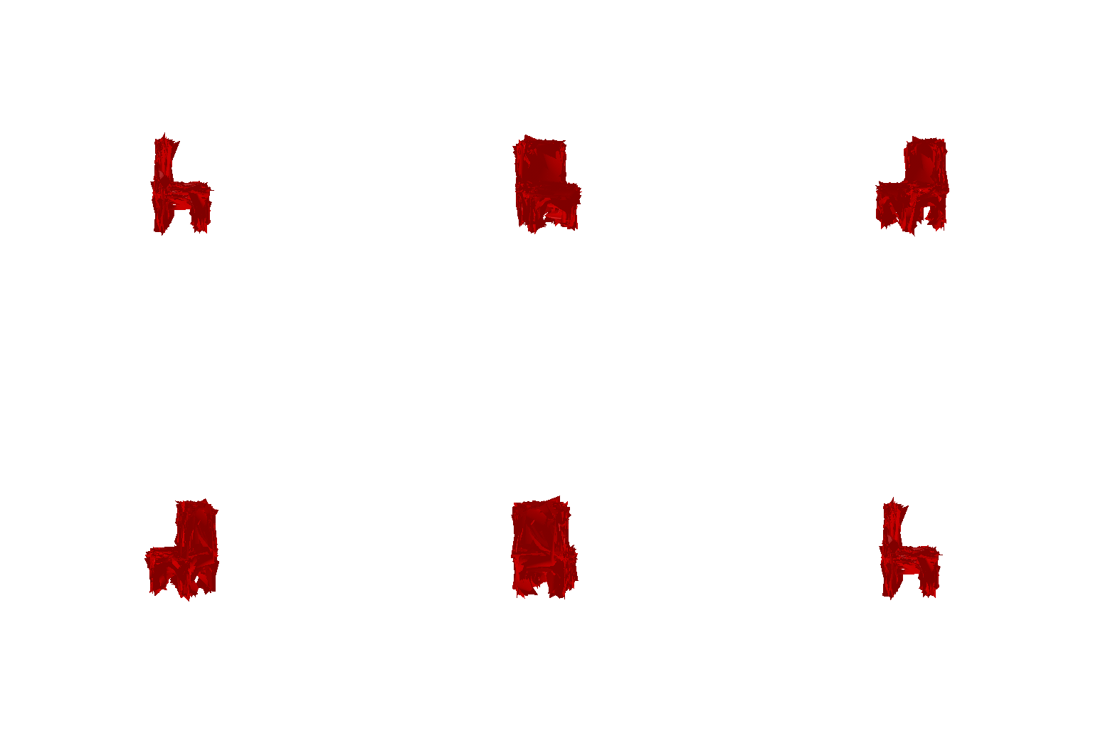
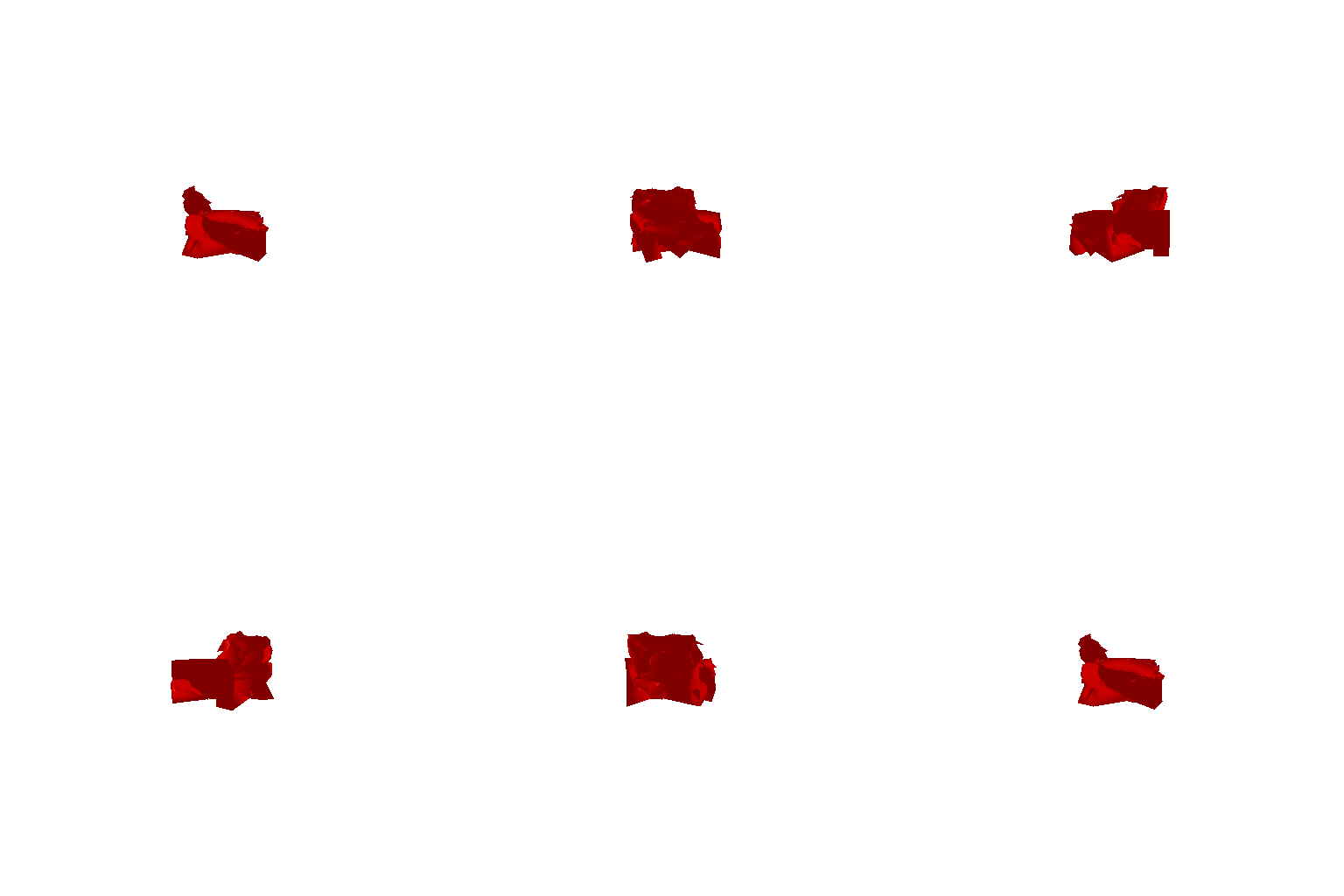
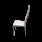
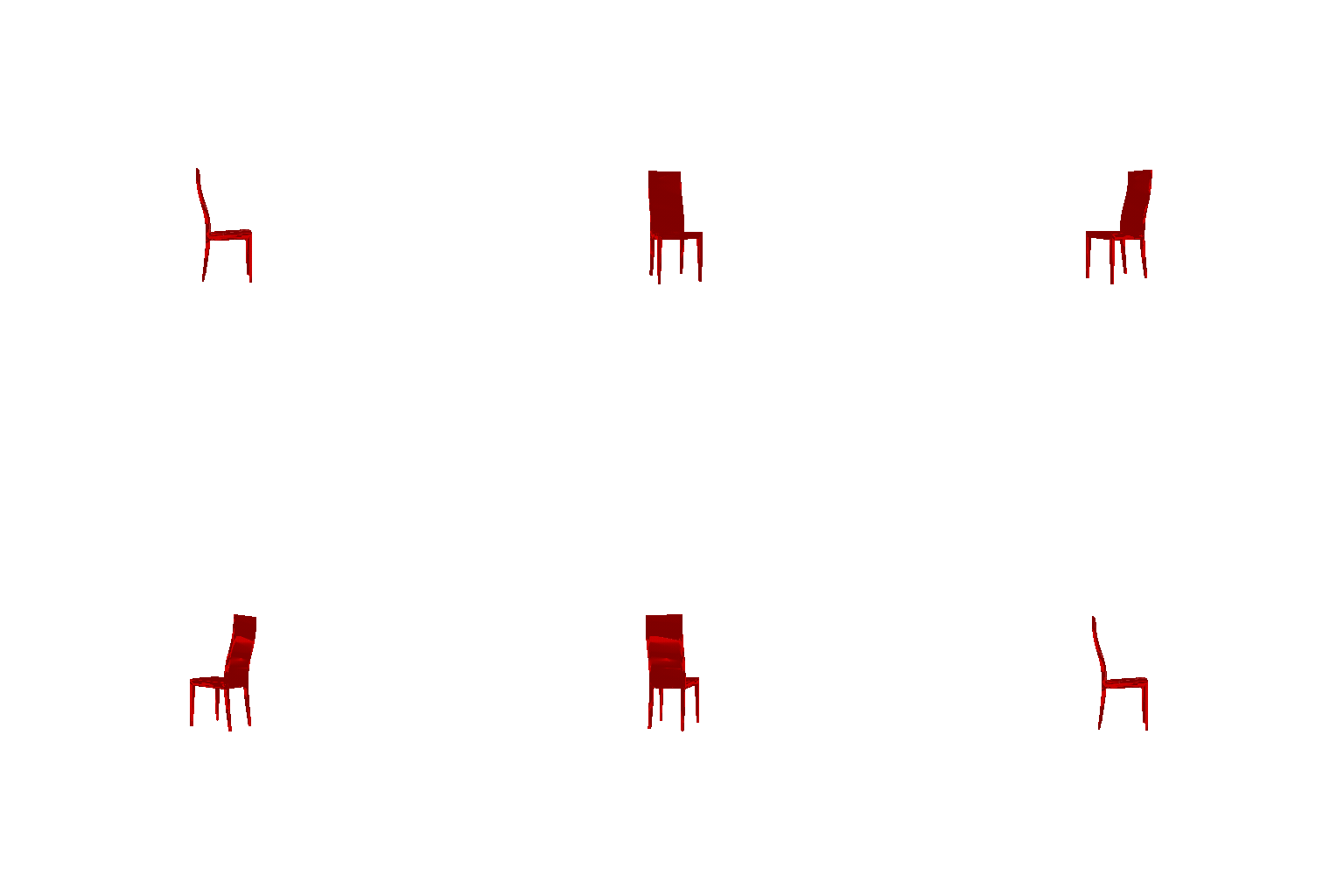
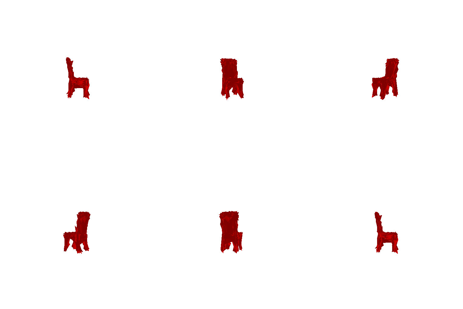
(##) 2.3 Image to mesh
| Image | Ground truth Mesh | Prediction (Voxel) |
|-----------------------|------------------------|------------------------|
| | | |
| | | |
| | | |
(##) 2.4 Quantitative comparisions
| F1 @ 0.05 | Graph | Average Score |
|-----------------------|------------------------|------------------------|
| F1 @ 0.05(VOX) | | 83.184 |
|F1 @ 0.05(POINT) | | 99.143 |
| F1 @ 0.05(MESH) | | 94.015 |
(###) Explanation
Here is a quantitative analysis of the 3 different representations
1. It was observed that F1 score for voxels at 0.05 threshold was the lowest compared to point clouds and mesh. This could be attributed to the fact that the grid size for the voxels was 32x32x32 and that resolution is not enough to capture all the fine details in the ground truth mesh.
2. Point clouds have near perfect F1 score because of their inherent property that they dont have connected edges. This gives them more flexibility while infering 3D from a single image.
3. Generating meshes were the most difficult to begin with because, they have strong connectivity between vertices. Hence they need stronger supervision. Using only point-based chamfer loss will result in pointy surfaces. A shape regularizer such as laplacian smoothening helps make the mesh smooth.
It was observed that both mesh and voxel models face challenges beyond simply accurately placing vertices in space, leading to lower average F1 scores. Additionally, it was found that certain chairs were easier to render than others. This can probably be attributed to the fact that chairs which closely resemble the typical or average chair in the dataset and are more frequently represented in the data are easier to render. However, both voxel and mesh models face difficulties in accurately modeling holes within the object.
(##) 2.5. Analyse effects of hyperparms variations
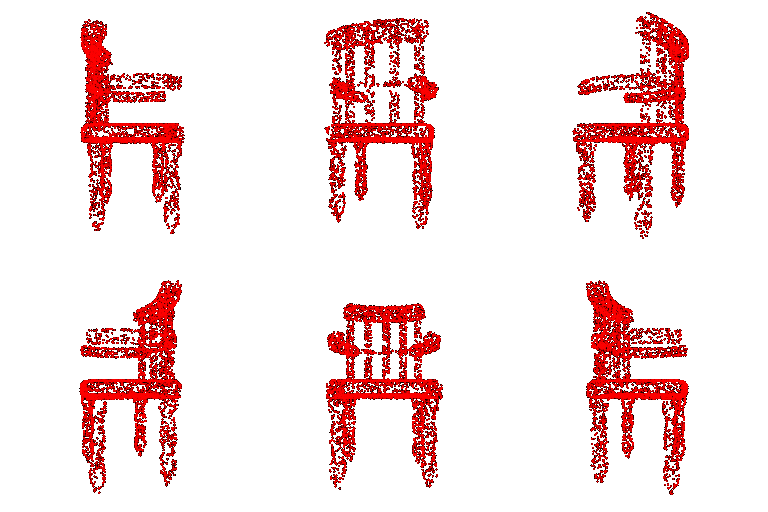
1. Reducing the number of points while training and evaluation (**n_point**)
I tried different number of points while training to see the effect both, qualitatively and quantatively.
When I changed the number of points from 5000 to 2500, I did not see a huge drop in F1 score. The score went from 94.0513 to 93.614
Visually the cloud looks much sparser than the one with 5000 points.
2. Mesh prediction by varying **w_chamfer** and **w_smooth**
Initially when I trained the model, I kept both these weights as 1.0 and got outputs which were pointy.
But later I realised that smoothing loss had to be increased to increase the mesh smoothness.
So I made the weight w_smooth as 5.0 and kept w_chamfer as 1.0. This resulted in more number of planes
being created which were all intersecting. Although the pointyness of the mesh reduced, it still looked bad.
So fix this, I altered the w_chamfer and made it 0.6 while keeping the smoothing weight the same as the previous
step. This got rid of the number of intersecting planes and made the output look decent.
I futher reduced w_chamfer and observed that the mesh improved over time.
So my insight was that, we need to balance between both these weights to improve over the mesh quality.
F1 score also improved with each of these iterative changes.
3. Increasing the mesh subdivision in **initial_mesh(ico_sphere)** from 4 to 5
The code provided to us used level 4 ico_sphere. I changed this to 5. this increased the number of faces and vertices
of the mesh. This process is called subdivision. Subdivision helped me improve the results qualitatively because, I could
now sample more points on a face and uniformly across faces. It was also observed that the F1 score increased nearly 5% after
subdivision.
Additionally, I also tried using torus as an initialization. It made the outputs worse. So I decided to stick with
ico_sphere level 5 and varied the smoothing and chamfer weights as mentioned in the previous point.
(##) 2.6. Interpret your model
(###) 1. **Visualization of confidence in different areas of the chair for voxels**
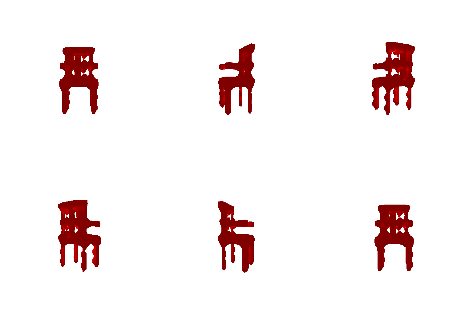
The visualization presented here depicts the predicted objects generated by the voxel method at varying isovalue levels.
It displays the level of confidence of the model in predicting different parts of the chair.
The results indicate that the model has the least confidence in predicting thinner features like legs,
and therefore a low isovalue is necessary to accurately capture the details of the chair.
However, even with this lower isovalue, the model's predictions for the legs are not entirely
accurate. On the other hand, the model is most confident in predicting the seat and backrest of the chair, as these features are common to most chairs.
| Vox (iso = 0) | Vox (iso = 0.1) |Vox (iso = 0.5)|
|-----------------------|------------------------|------------------------|
| | | |
| | | |
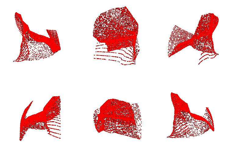
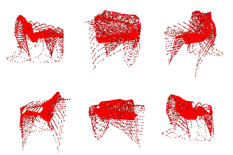
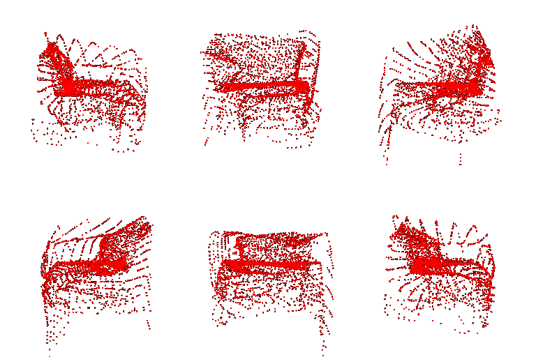
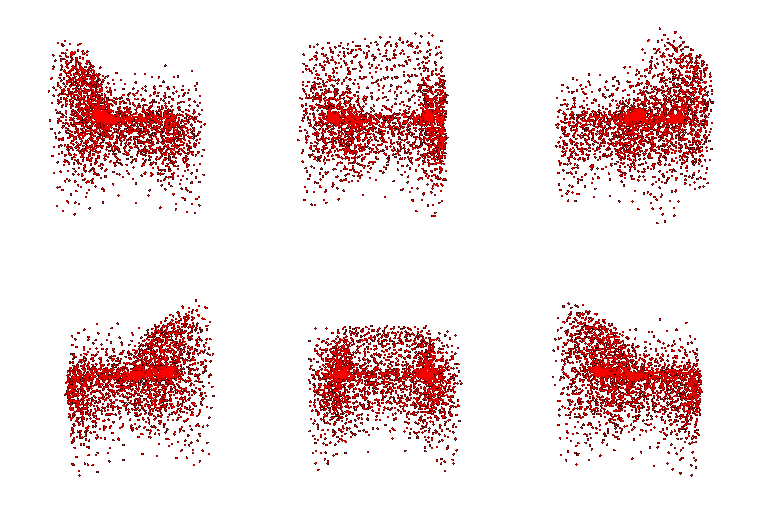
(###) 2. **What does the model learn over time?**
Here I try to visualize what a model learns over time. I keep the camera in a fixed place and capture an image every 100 iterations to see what the model is learning over time.
As an example I try to visualize only a mesh but the idea remains the same for all representations
It can be seen that initially the model makes a rough estimate of different planes in the mesh. Over time as loss decreases, it understands about the different weights assigned in the model, w_chamfer
and w_smooth and thereby adjusts the mesh accordingly.
| Mesh evolution over time |
|-----|---|
| |
**Parametric representation evolution over time**
|Iter 200 | Iter 1300 | Iter 5000 | Iter 18000 |
|---|---|---|---|---|
| ||||
(#) 3. Exploring some recent architectures.
I implemented an occupancy network which was inspired by the architecture mentioned in this.(paper). The architecture encodes a 3D point and an input image(of the same object) and then that global feature vector is then passed to a neural net to get an occupancy value.
Similarly, the parametric network architecture was inspired by the AtlasNet paper. The architecture encodes an image and randomly sampled 2D points and outputs their 3D points. The global feature vector is a combination of both image and the 2D point.
(##) 3.1 Implicit network
The implicit network architecture I used is described below
1. ResNet18 was used as a feature encoder for images. The feature vector size was restricted to 512
2. Sample n_points from ground truth data and pass it into a point encoder to generate a feature vector of size 512
3. Concatenate both the feature vectors to obtain a global feature vector.
4. Feed this global feature vector into conditonal batch norm decoder, similar to what is being done in the original paper
The loss function here remains the same like in case of voxels. We use BCEwithLogitsLoss
| F1 @ 0.05 | Graph | Average Score |
|-----------------------|------------------------|------------------------|
| F1 @ 0.05 (IMPLICIT) | | 81.677 |
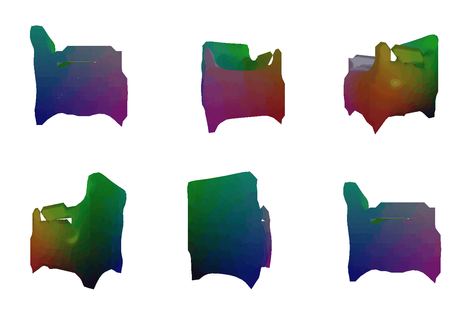
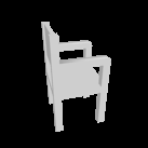
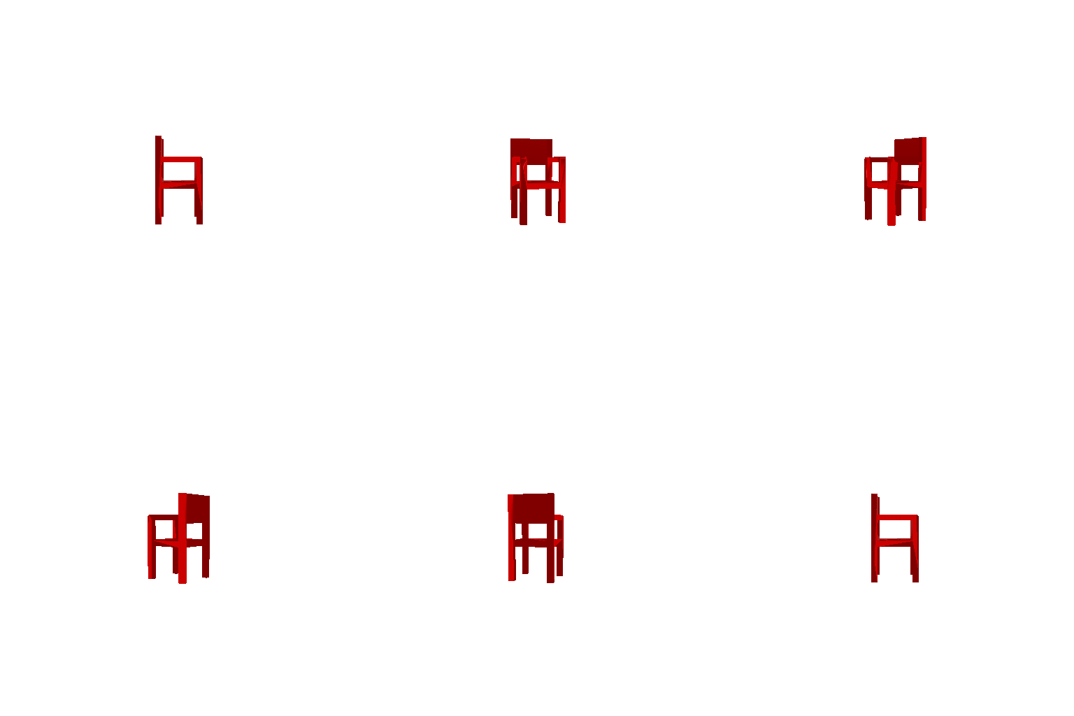
| Image | Ground truth Mesh | Prediction (Implicit representation) |
|-----------------------|------------------------|------------------------|
| | | |
| | | |
(##) 3.2 Parametric network
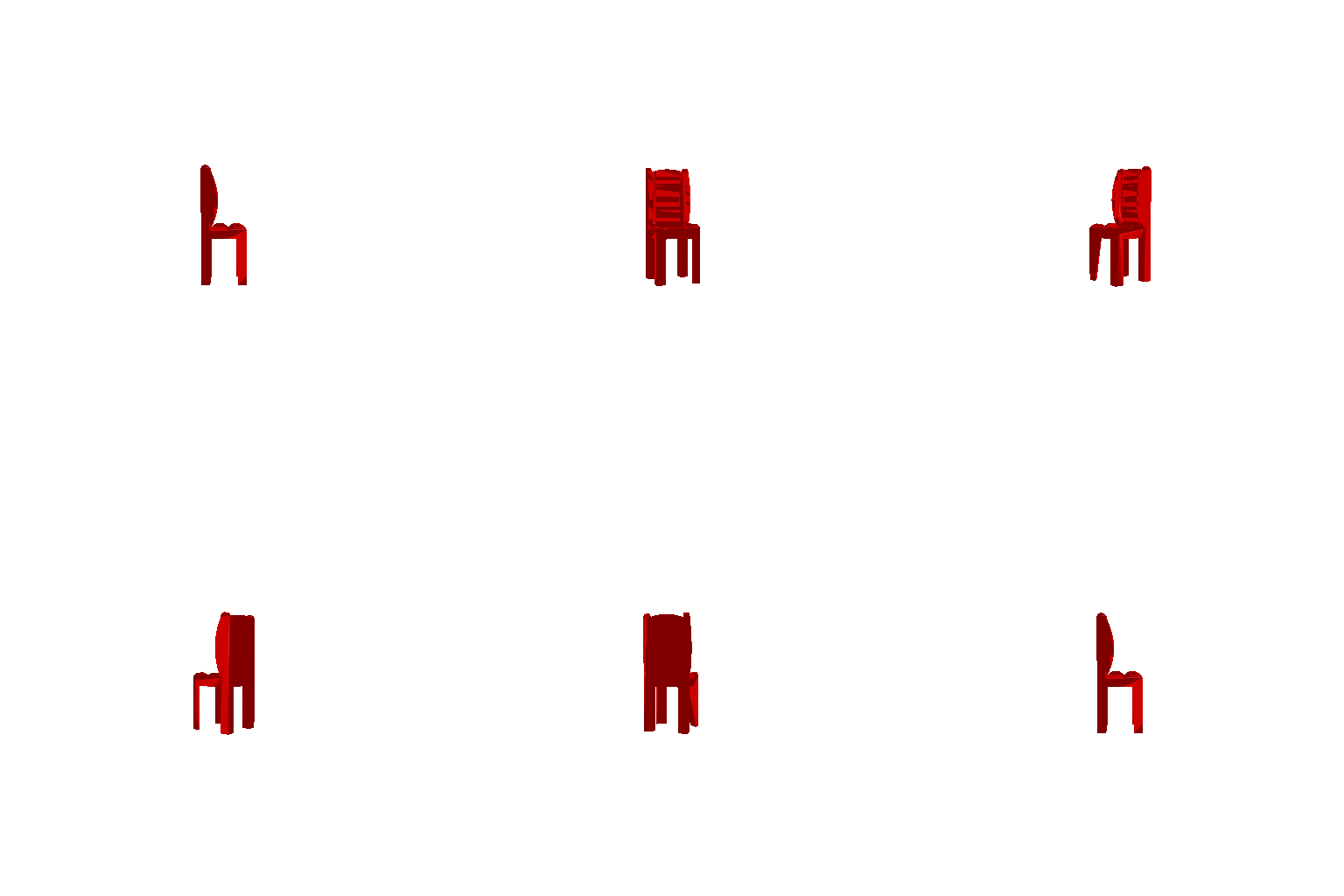
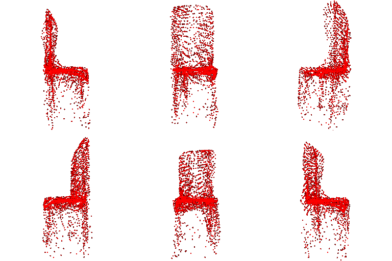
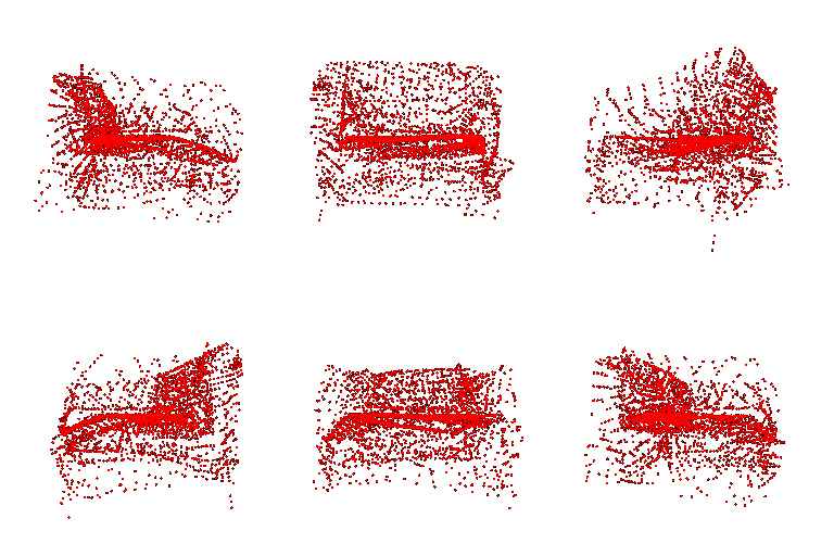
The parametric network architecture as follows
1. ResNet18 was used as a feature encoder for images. The feature vector size was restricted to 128
2. Randomly sample 2D points from a surface by defining a grid. We pass these points through a linear feature encoder to encode points into a feature vector of size 128
3. We then add both feature vectors to obtain a combined feature vector
4. The global feature vector is then passed through the decoder to obtain a predicted point cloud
The loss function remains the same as in case of point cloud training
| F1 @ 0.05 | Graph | Average Score |
|-----------------------|------------------------|------------------------|
| F1 @ 0.05 (PARAMETRIC) | | 93.625 |
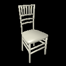
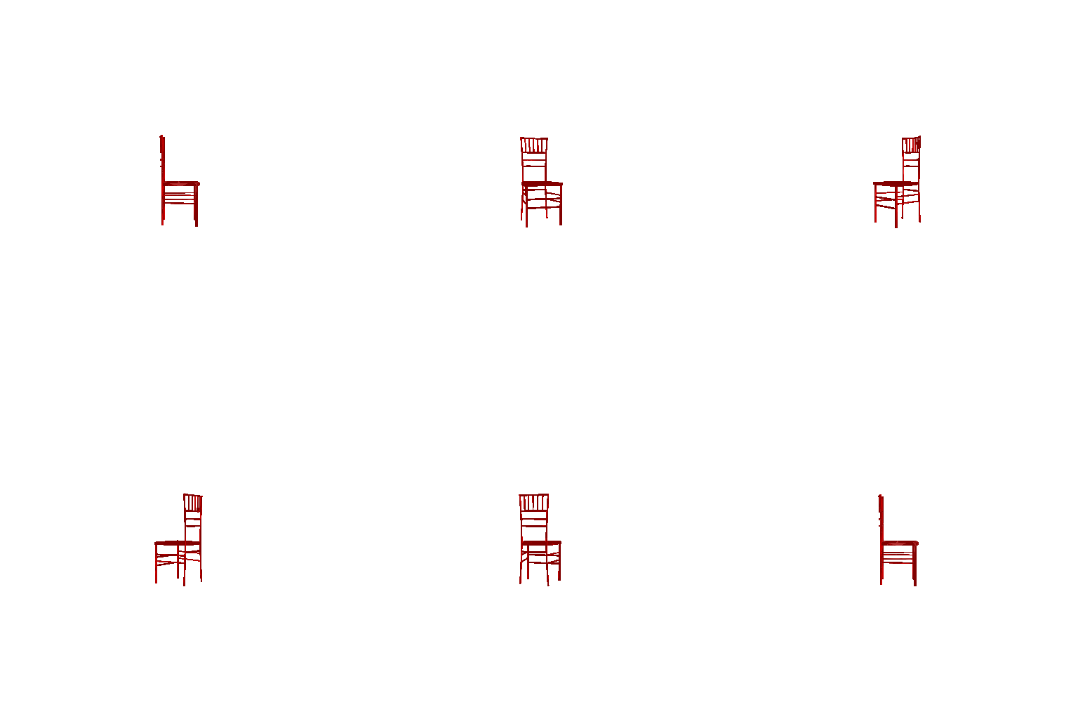
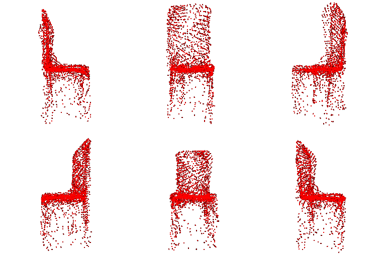
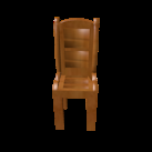
| Image | Ground truth Mesh | Prediction (Paramertic point cloud) |
|-----------------------|------------------------|------------------------|
| | | |
| | | |
| | | |
 (#) 1. Exploring loss functions
This section will involve defining a loss function, for fitting voxels, point clouds and meshes.
(##) 1.1. Fitting a voxel grid
| Voxel Target | Voxel Optimized |
|-----------------------|------------------------|
|
(#) 1. Exploring loss functions
This section will involve defining a loss function, for fitting voxels, point clouds and meshes.
(##) 1.1. Fitting a voxel grid
| Voxel Target | Voxel Optimized |
|-----------------------|------------------------|
| |
| |
|
|
| |
| |
|
|
| |
| |
(##) 1.2. Fitting a point cloud
| Pointcloud Target | Pointcloud Optimized |
|-----------------------|------------------------|
|
|
(##) 1.2. Fitting a point cloud
| Pointcloud Target | Pointcloud Optimized |
|-----------------------|------------------------|
| |
| |
|
|
| |
| |
|
|
| |
| |
(##) 1.3. Fitting a mesh
| Mesh Target | Mesh Optimized |
|-----------------------|------------------------|
|
|
(##) 1.3. Fitting a mesh
| Mesh Target | Mesh Optimized |
|-----------------------|------------------------|
| |
| |
|
|
| |
| |
|
|
| |
| |
(#) 2. Practicing with Meshes
(##) 2.1 Image to voxel grid
| Image | Ground truth Mesh | Prediction (Voxel) |
|-----------------------|------------------------|------------------------|
|
|
(#) 2. Practicing with Meshes
(##) 2.1 Image to voxel grid
| Image | Ground truth Mesh | Prediction (Voxel) |
|-----------------------|------------------------|------------------------|
| |
| |
|  |
|
|
| |
| |
|  |
|
|
| |
| |
|  |
(##) 2.2 Image to point cloud
| Image | Ground truth Mesh | Prediction (Point cloud) |
|-----------------------|------------------------|------------------------|
|
|
(##) 2.2 Image to point cloud
| Image | Ground truth Mesh | Prediction (Point cloud) |
|-----------------------|------------------------|------------------------|
| |
| |
|  |
|
|
| |
|
|
| |
(##) 2.3 Image to mesh
| Image | Ground truth Mesh | Prediction (Voxel) |
|-----------------------|------------------------|------------------------|
|
|
(##) 2.3 Image to mesh
| Image | Ground truth Mesh | Prediction (Voxel) |
|-----------------------|------------------------|------------------------|
| |
|
|
| |
|
|
| |
| |
|  |
(##) 2.4 Quantitative comparisions
| F1 @ 0.05 | Graph | Average Score |
|-----------------------|------------------------|------------------------|
| F1 @ 0.05(VOX) |
|
(##) 2.4 Quantitative comparisions
| F1 @ 0.05 | Graph | Average Score |
|-----------------------|------------------------|------------------------|
| F1 @ 0.05(VOX) | 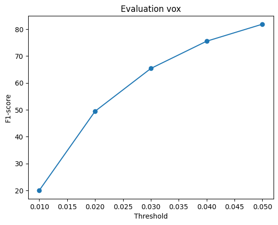 | 83.184 |
|F1 @ 0.05(POINT) |
| 83.184 |
|F1 @ 0.05(POINT) | 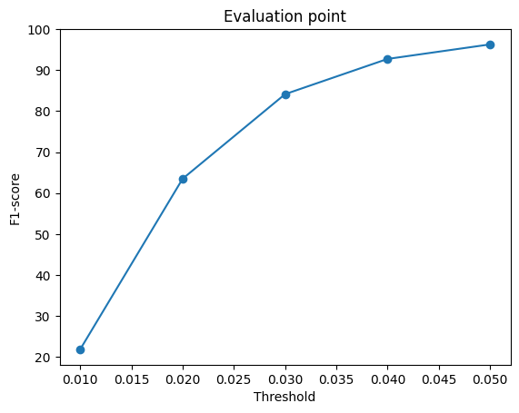 | 99.143 |
| F1 @ 0.05(MESH) |
| 99.143 |
| F1 @ 0.05(MESH) | 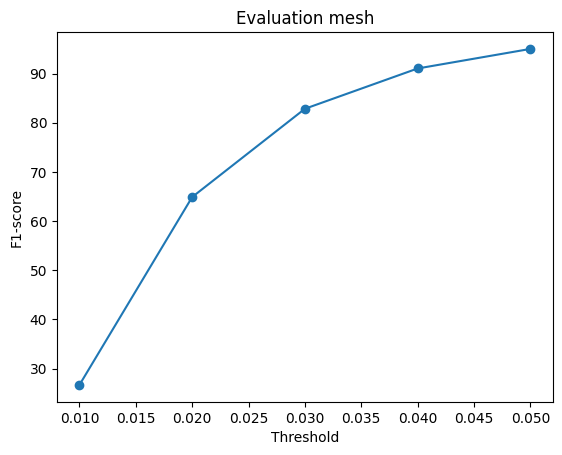 | 94.015 |
(###) Explanation
Here is a quantitative analysis of the 3 different representations
1. It was observed that F1 score for voxels at 0.05 threshold was the lowest compared to point clouds and mesh. This could be attributed to the fact that the grid size for the voxels was 32x32x32 and that resolution is not enough to capture all the fine details in the ground truth mesh.
2. Point clouds have near perfect F1 score because of their inherent property that they dont have connected edges. This gives them more flexibility while infering 3D from a single image.
3. Generating meshes were the most difficult to begin with because, they have strong connectivity between vertices. Hence they need stronger supervision. Using only point-based chamfer loss will result in pointy surfaces. A shape regularizer such as laplacian smoothening helps make the mesh smooth.
It was observed that both mesh and voxel models face challenges beyond simply accurately placing vertices in space, leading to lower average F1 scores. Additionally, it was found that certain chairs were easier to render than others. This can probably be attributed to the fact that chairs which closely resemble the typical or average chair in the dataset and are more frequently represented in the data are easier to render. However, both voxel and mesh models face difficulties in accurately modeling holes within the object.
(##) 2.5. Analyse effects of hyperparms variations
1. Reducing the number of points while training and evaluation (**n_point**)
I tried different number of points while training to see the effect both, qualitatively and quantatively.
When I changed the number of points from 5000 to 2500, I did not see a huge drop in F1 score. The score went from 94.0513 to 93.614
Visually the cloud looks much sparser than the one with 5000 points.
2. Mesh prediction by varying **w_chamfer** and **w_smooth**
Initially when I trained the model, I kept both these weights as 1.0 and got outputs which were pointy.
But later I realised that smoothing loss had to be increased to increase the mesh smoothness.
So I made the weight w_smooth as 5.0 and kept w_chamfer as 1.0. This resulted in more number of planes
being created which were all intersecting. Although the pointyness of the mesh reduced, it still looked bad.
So fix this, I altered the w_chamfer and made it 0.6 while keeping the smoothing weight the same as the previous
step. This got rid of the number of intersecting planes and made the output look decent.
I futher reduced w_chamfer and observed that the mesh improved over time.
So my insight was that, we need to balance between both these weights to improve over the mesh quality.
F1 score also improved with each of these iterative changes.
3. Increasing the mesh subdivision in **initial_mesh(ico_sphere)** from 4 to 5
The code provided to us used level 4 ico_sphere. I changed this to 5. this increased the number of faces and vertices
of the mesh. This process is called subdivision. Subdivision helped me improve the results qualitatively because, I could
now sample more points on a face and uniformly across faces. It was also observed that the F1 score increased nearly 5% after
subdivision.
Additionally, I also tried using torus as an initialization. It made the outputs worse. So I decided to stick with
ico_sphere level 5 and varied the smoothing and chamfer weights as mentioned in the previous point.
(##) 2.6. Interpret your model
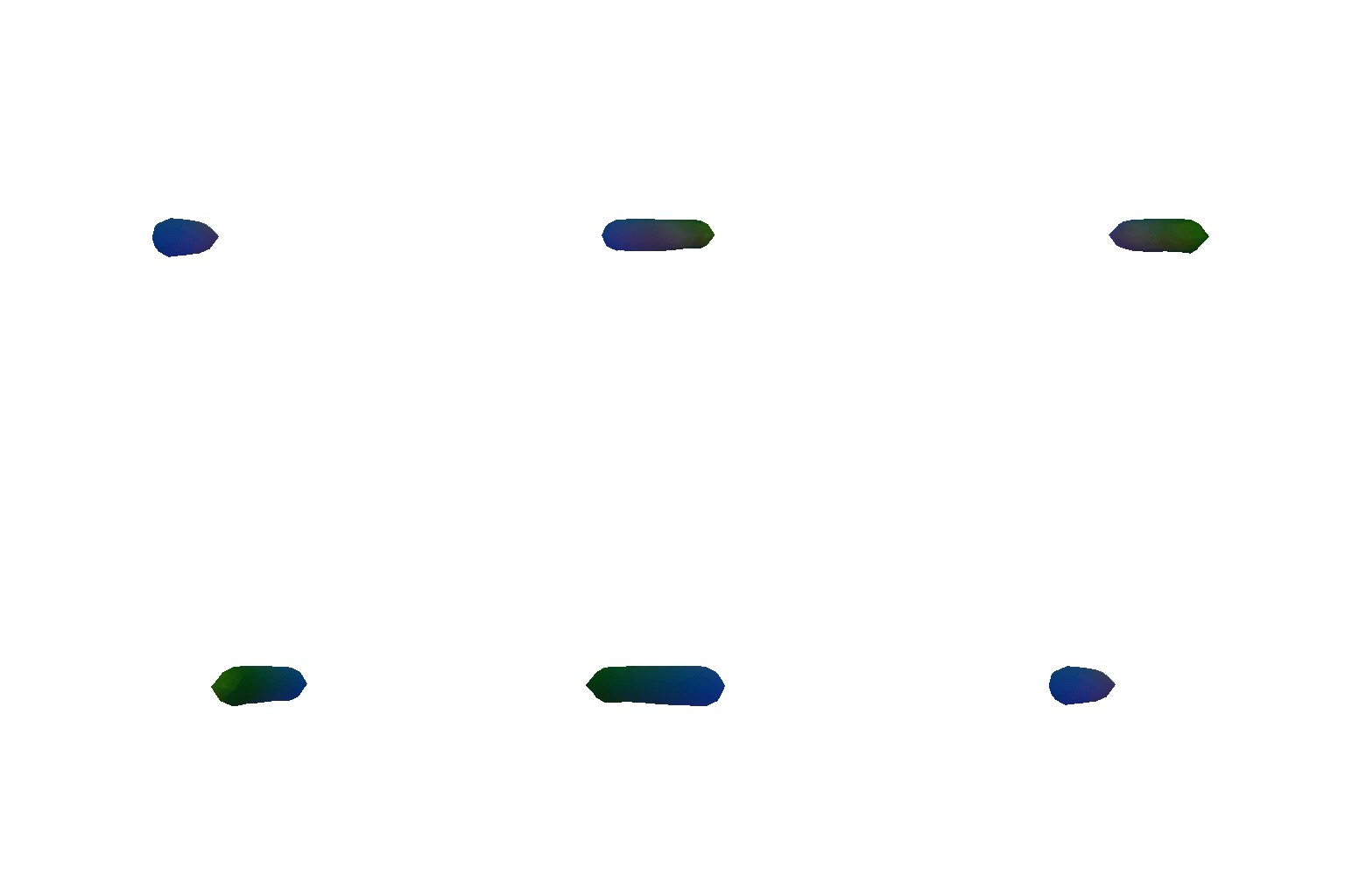
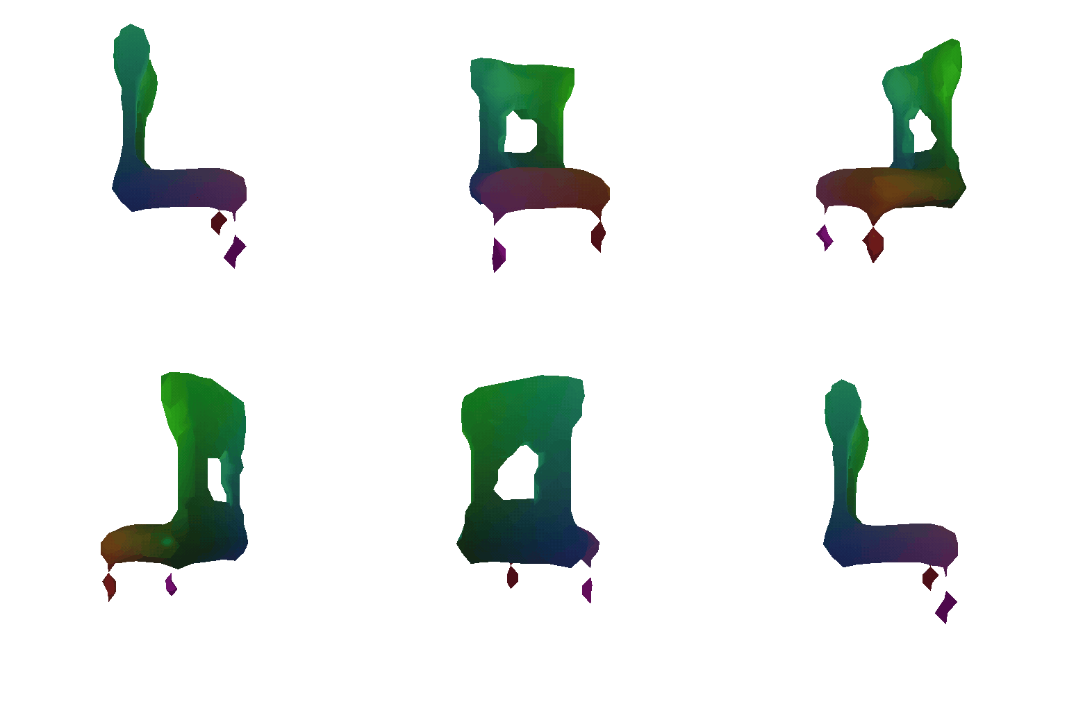
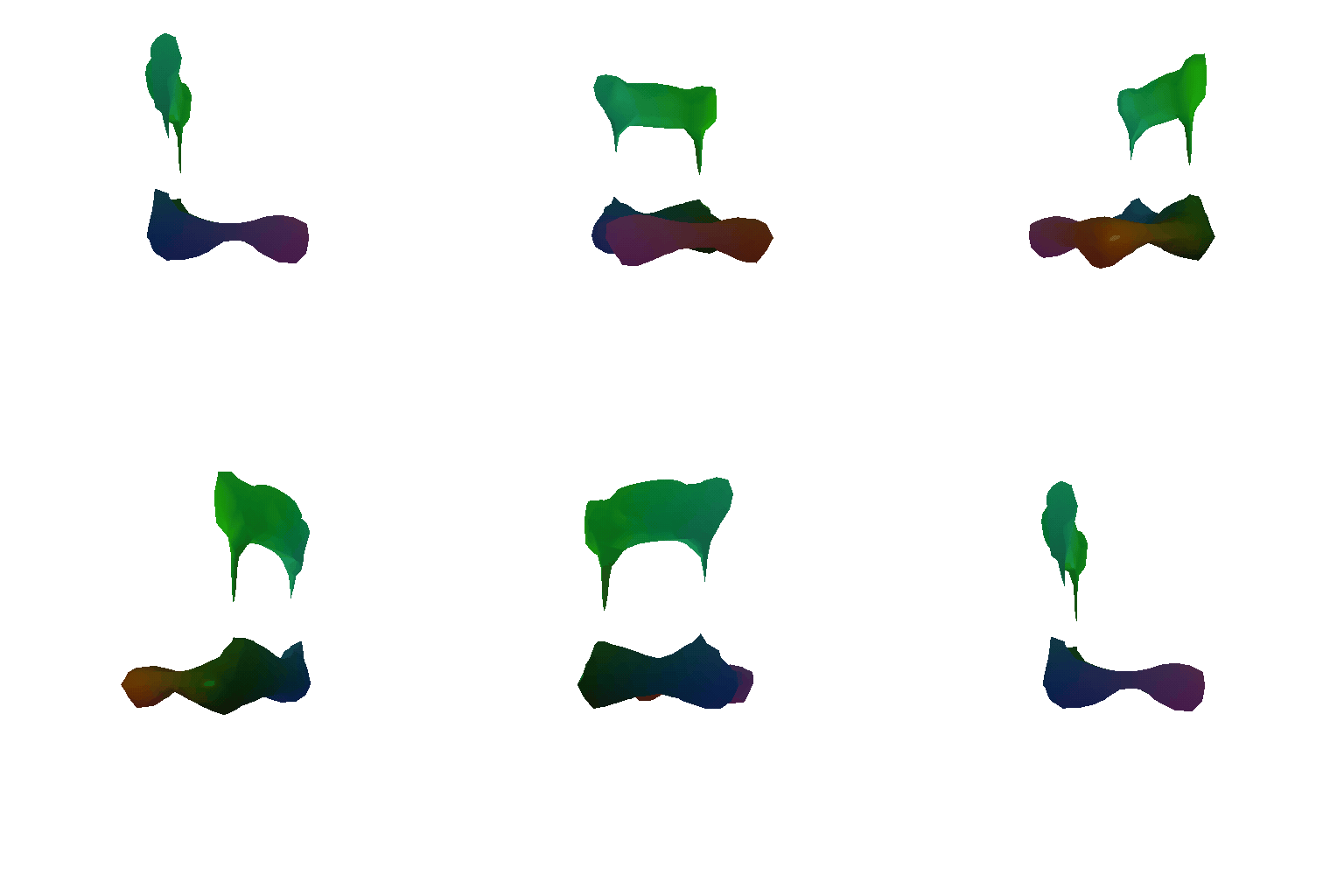
(###) 1. **Visualization of confidence in different areas of the chair for voxels**
The visualization presented here depicts the predicted objects generated by the voxel method at varying isovalue levels.
It displays the level of confidence of the model in predicting different parts of the chair.
The results indicate that the model has the least confidence in predicting thinner features like legs,
and therefore a low isovalue is necessary to accurately capture the details of the chair.
However, even with this lower isovalue, the model's predictions for the legs are not entirely
accurate. On the other hand, the model is most confident in predicting the seat and backrest of the chair, as these features are common to most chairs.
| Vox (iso = 0) | Vox (iso = 0.1) |Vox (iso = 0.5)|
|-----------------------|------------------------|------------------------|
|
| 94.015 |
(###) Explanation
Here is a quantitative analysis of the 3 different representations
1. It was observed that F1 score for voxels at 0.05 threshold was the lowest compared to point clouds and mesh. This could be attributed to the fact that the grid size for the voxels was 32x32x32 and that resolution is not enough to capture all the fine details in the ground truth mesh.
2. Point clouds have near perfect F1 score because of their inherent property that they dont have connected edges. This gives them more flexibility while infering 3D from a single image.
3. Generating meshes were the most difficult to begin with because, they have strong connectivity between vertices. Hence they need stronger supervision. Using only point-based chamfer loss will result in pointy surfaces. A shape regularizer such as laplacian smoothening helps make the mesh smooth.
It was observed that both mesh and voxel models face challenges beyond simply accurately placing vertices in space, leading to lower average F1 scores. Additionally, it was found that certain chairs were easier to render than others. This can probably be attributed to the fact that chairs which closely resemble the typical or average chair in the dataset and are more frequently represented in the data are easier to render. However, both voxel and mesh models face difficulties in accurately modeling holes within the object.
(##) 2.5. Analyse effects of hyperparms variations
1. Reducing the number of points while training and evaluation (**n_point**)
I tried different number of points while training to see the effect both, qualitatively and quantatively.
When I changed the number of points from 5000 to 2500, I did not see a huge drop in F1 score. The score went from 94.0513 to 93.614
Visually the cloud looks much sparser than the one with 5000 points.
2. Mesh prediction by varying **w_chamfer** and **w_smooth**
Initially when I trained the model, I kept both these weights as 1.0 and got outputs which were pointy.
But later I realised that smoothing loss had to be increased to increase the mesh smoothness.
So I made the weight w_smooth as 5.0 and kept w_chamfer as 1.0. This resulted in more number of planes
being created which were all intersecting. Although the pointyness of the mesh reduced, it still looked bad.
So fix this, I altered the w_chamfer and made it 0.6 while keeping the smoothing weight the same as the previous
step. This got rid of the number of intersecting planes and made the output look decent.
I futher reduced w_chamfer and observed that the mesh improved over time.
So my insight was that, we need to balance between both these weights to improve over the mesh quality.
F1 score also improved with each of these iterative changes.
3. Increasing the mesh subdivision in **initial_mesh(ico_sphere)** from 4 to 5
The code provided to us used level 4 ico_sphere. I changed this to 5. this increased the number of faces and vertices
of the mesh. This process is called subdivision. Subdivision helped me improve the results qualitatively because, I could
now sample more points on a face and uniformly across faces. It was also observed that the F1 score increased nearly 5% after
subdivision.
Additionally, I also tried using torus as an initialization. It made the outputs worse. So I decided to stick with
ico_sphere level 5 and varied the smoothing and chamfer weights as mentioned in the previous point.
(##) 2.6. Interpret your model
(###) 1. **Visualization of confidence in different areas of the chair for voxels**
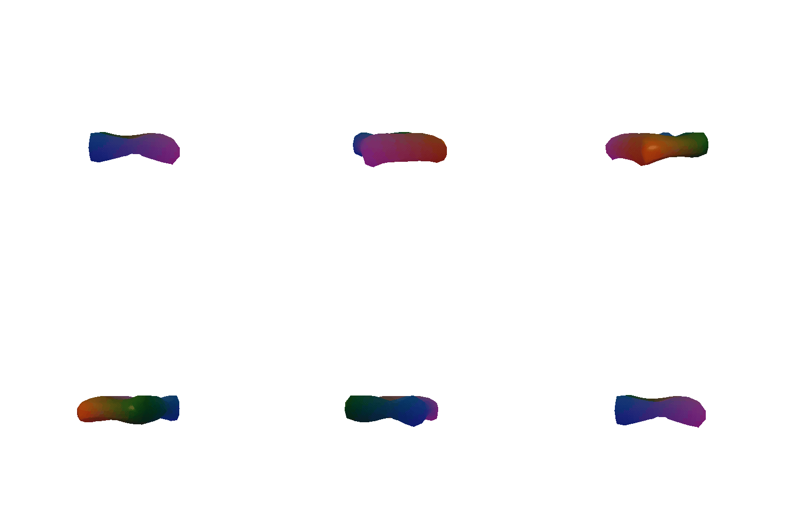
The visualization presented here depicts the predicted objects generated by the voxel method at varying isovalue levels.
It displays the level of confidence of the model in predicting different parts of the chair.
The results indicate that the model has the least confidence in predicting thinner features like legs,
and therefore a low isovalue is necessary to accurately capture the details of the chair.
However, even with this lower isovalue, the model's predictions for the legs are not entirely
accurate. On the other hand, the model is most confident in predicting the seat and backrest of the chair, as these features are common to most chairs.
| Vox (iso = 0) | Vox (iso = 0.1) |Vox (iso = 0.5)|
|-----------------------|------------------------|------------------------|
| |
| |
|  |
|
|
| |
| |
|  |
(###) 2. **What does the model learn over time?**
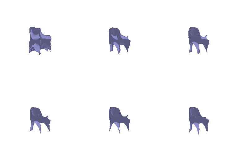
Here I try to visualize what a model learns over time. I keep the camera in a fixed place and capture an image every 100 iterations to see what the model is learning over time.
As an example I try to visualize only a mesh but the idea remains the same for all representations
It can be seen that initially the model makes a rough estimate of different planes in the mesh. Over time as loss decreases, it understands about the different weights assigned in the model, w_chamfer
and w_smooth and thereby adjusts the mesh accordingly.
| Mesh evolution over time |
|-----|---|
|
|
(###) 2. **What does the model learn over time?**
Here I try to visualize what a model learns over time. I keep the camera in a fixed place and capture an image every 100 iterations to see what the model is learning over time.
As an example I try to visualize only a mesh but the idea remains the same for all representations
It can be seen that initially the model makes a rough estimate of different planes in the mesh. Over time as loss decreases, it understands about the different weights assigned in the model, w_chamfer
and w_smooth and thereby adjusts the mesh accordingly.
| Mesh evolution over time |
|-----|---|
| |
**Parametric representation evolution over time**
|Iter 200 | Iter 1300 | Iter 5000 | Iter 18000 |
|---|---|---|---|---|
|
|
**Parametric representation evolution over time**
|Iter 200 | Iter 1300 | Iter 5000 | Iter 18000 |
|---|---|---|---|---|
| |
| |
| |
| |
(#) 3. Exploring some recent architectures.
I implemented an occupancy network which was inspired by the architecture mentioned in this.(paper). The architecture encodes a 3D point and an input image(of the same object) and then that global feature vector is then passed to a neural net to get an occupancy value.
Similarly, the parametric network architecture was inspired by the AtlasNet paper. The architecture encodes an image and randomly sampled 2D points and outputs their 3D points. The global feature vector is a combination of both image and the 2D point.
(##) 3.1 Implicit network
The implicit network architecture I used is described below
1. ResNet18 was used as a feature encoder for images. The feature vector size was restricted to 512
2. Sample n_points from ground truth data and pass it into a point encoder to generate a feature vector of size 512
3. Concatenate both the feature vectors to obtain a global feature vector.
4. Feed this global feature vector into conditonal batch norm decoder, similar to what is being done in the original paper
The loss function here remains the same like in case of voxels. We use BCEwithLogitsLoss
| F1 @ 0.05 | Graph | Average Score |
|-----------------------|------------------------|------------------------|
| F1 @ 0.05 (IMPLICIT) |
|
(#) 3. Exploring some recent architectures.
I implemented an occupancy network which was inspired by the architecture mentioned in this.(paper). The architecture encodes a 3D point and an input image(of the same object) and then that global feature vector is then passed to a neural net to get an occupancy value.
Similarly, the parametric network architecture was inspired by the AtlasNet paper. The architecture encodes an image and randomly sampled 2D points and outputs their 3D points. The global feature vector is a combination of both image and the 2D point.
(##) 3.1 Implicit network
The implicit network architecture I used is described below
1. ResNet18 was used as a feature encoder for images. The feature vector size was restricted to 512
2. Sample n_points from ground truth data and pass it into a point encoder to generate a feature vector of size 512
3. Concatenate both the feature vectors to obtain a global feature vector.
4. Feed this global feature vector into conditonal batch norm decoder, similar to what is being done in the original paper
The loss function here remains the same like in case of voxels. We use BCEwithLogitsLoss
| F1 @ 0.05 | Graph | Average Score |
|-----------------------|------------------------|------------------------|
| F1 @ 0.05 (IMPLICIT) | 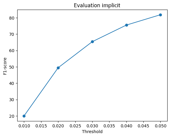 | 81.677 |
| Image | Ground truth Mesh | Prediction (Implicit representation) |
|-----------------------|------------------------|------------------------|
|
| 81.677 |
| Image | Ground truth Mesh | Prediction (Implicit representation) |
|-----------------------|------------------------|------------------------|
| |
| |
|  |
|
|
| |
| |
|  |
(##) 3.2 Parametric network
The parametric network architecture as follows
1. ResNet18 was used as a feature encoder for images. The feature vector size was restricted to 128
2. Randomly sample 2D points from a surface by defining a grid. We pass these points through a linear feature encoder to encode points into a feature vector of size 128
3. We then add both feature vectors to obtain a combined feature vector
4. The global feature vector is then passed through the decoder to obtain a predicted point cloud
The loss function remains the same as in case of point cloud training
| F1 @ 0.05 | Graph | Average Score |
|-----------------------|------------------------|------------------------|
| F1 @ 0.05 (PARAMETRIC) |
|
(##) 3.2 Parametric network
The parametric network architecture as follows
1. ResNet18 was used as a feature encoder for images. The feature vector size was restricted to 128
2. Randomly sample 2D points from a surface by defining a grid. We pass these points through a linear feature encoder to encode points into a feature vector of size 128
3. We then add both feature vectors to obtain a combined feature vector
4. The global feature vector is then passed through the decoder to obtain a predicted point cloud
The loss function remains the same as in case of point cloud training
| F1 @ 0.05 | Graph | Average Score |
|-----------------------|------------------------|------------------------|
| F1 @ 0.05 (PARAMETRIC) | 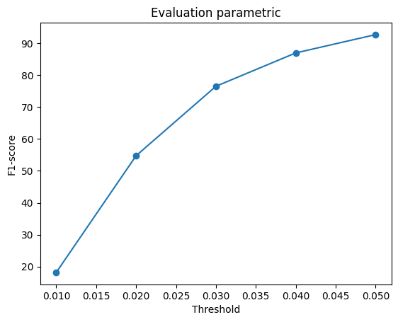 | 93.625 |
| Image | Ground truth Mesh | Prediction (Paramertic point cloud) |
|-----------------------|------------------------|------------------------|
|
| 93.625 |
| Image | Ground truth Mesh | Prediction (Paramertic point cloud) |
|-----------------------|------------------------|------------------------|
| |
| |
|  |
|
|
| |
| |
|  |
|
|
| |
| |
|  |
|