**Cats Meets GANs**
Student name: Abhishek Pavani
(##) LATE DAYS : 0
(#) **DEPENDENCY INSTALLATION**
(##) Install conda environment by running
`conda create --name geometry-based-methods`
(##) To install packages
`conda install -r requirements.txt`
(#) **RUN CODE**
(##) To run code for Q1(a) and see the computed F matrix and E matrix using 8 point algorithm, run
`python main.py --question='q1a' --object='chair'`
`python main.py --question='q1a' --object='teddy'`
(##) To run code for Q1(b) and see the computed F matrix and E matrix using 7 point algorithm, run
`python main.py --question='q1b' --object='toybus'`
`python main.py --question='q1b' --object='toytrain'`
(##) To run code for Q2 and see the computed F matrix 8 point RANSAC algorithm, run
`python main.py --question='q2' --object='chair' --num_points=8`
`python main.py --question='q2' --object='teddy' --num_points=8`
(##) To run code for Q2 and see the computed F matrix 7 point RANSAC algorithm, run
`python main.py --question='q2' --object='toybus' --num_points=7`
`python main.py --question='q2' --object='toytrain' --num_points=7`
(##) To traingulate points and see them in 3D, run
`python main.py --question='q3'`
(##) To perform bundle adjustment, run
`python main.py --question='q4'`
(##) To see fundamental matrix estimation on own images,run
`python main.py --question='q5'`
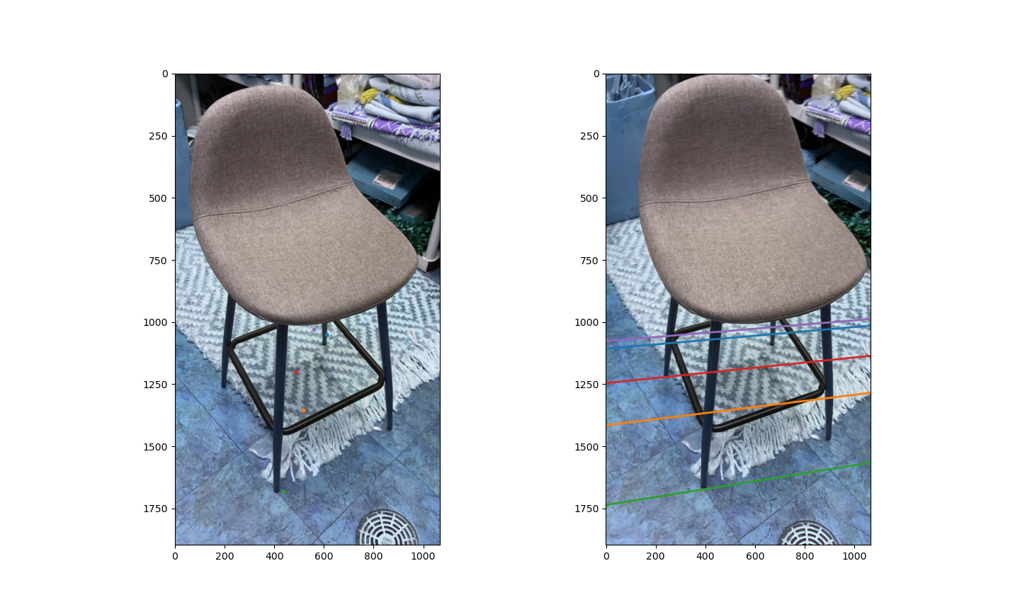
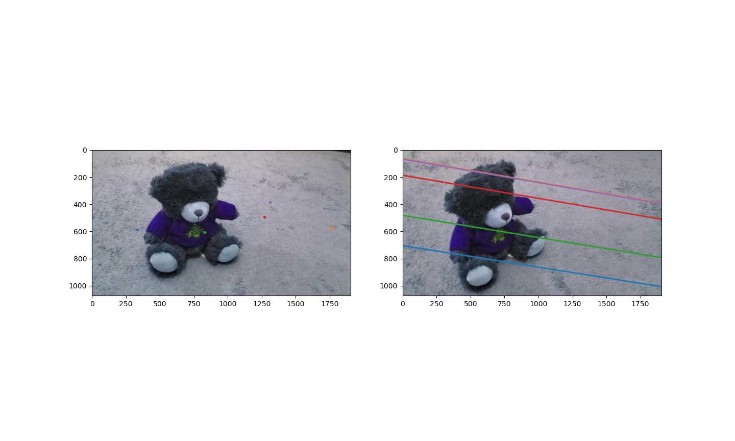
(#) Q1A(1) 8-point Algorithm.
(##) RESULTS
(##) BRIEF EXPLANATION OF IMPLEMENTATION
1. Given the points, first step is to normalize them
2. Normalize these points using the transforamtion matrix below
T= $\begin{bmatrix}
s & 0 & -s*x_{0} \\
0 & s & -s*y_{0} \\
0 & 0 & 1
\end{bmatrix}$
3. Using these normalized coordinates, construct a matrix to recover the fundamental matrix. This can be done using the epipolar constraint $x'^{T} F x =0$
4. Using the above equation we can reduce it to the form Af = 0, where f contains all elements of the fundamental matrix and A is constructed as follows
A = $\begin{bmatrix}
x_{1}*x_{2} & x_{2}*y_{1} & x_{2} & y_{2}*x_{1} & y_{1}*y_{2} & y_{2} & x_{1} & y_{1} & 1
\end{bmatrix}$
Each point-point correspondence will give one such equation and we need 8 such equations to solve for all elements of F
Note: here I used all correspondences as suggested in the piazza post instead of using only 8 points.
5. Now perform SVD to recover all elements of F
6. Once we get F, we first unnormilize the F matrix using $F_{unnormalized} = T'^{T} F_{normalized} T$ . After this, we set the last element to one and also enforce rank 2 constraint. We can do this by setting $\sigma_{3} = 0$
7. After we enforce rank 2 constraint, we again compute F by multiplying u, s and v
(#) Q1A(2).
(##) RESULTS
$E_{chair}$ = $\begin{bmatrix}
0.11320053 & 1.83773515 & 1.0941499 \\
-2.72837156 & 0.26432516 & 16.0267316 \\
-2.72725279 &-16.09946177 & 0.44957708 \\
\end{bmatrix}$
$E_{teddy}$ = $\begin{bmatrix}
0.13499427& -0.04854368& 0.79742868 \\
-0.52647433& -0.33213843& -4.66435097 \\
-1.93860455& 4.53037473& -0.02513974
\end{bmatrix}$
(##) BRIEF EXPLANATION OF IMPLEMENTATION
1. Once you compute F using 8 point algorithm, E can be estimated using the following expression, $E = K'^{T} F K$
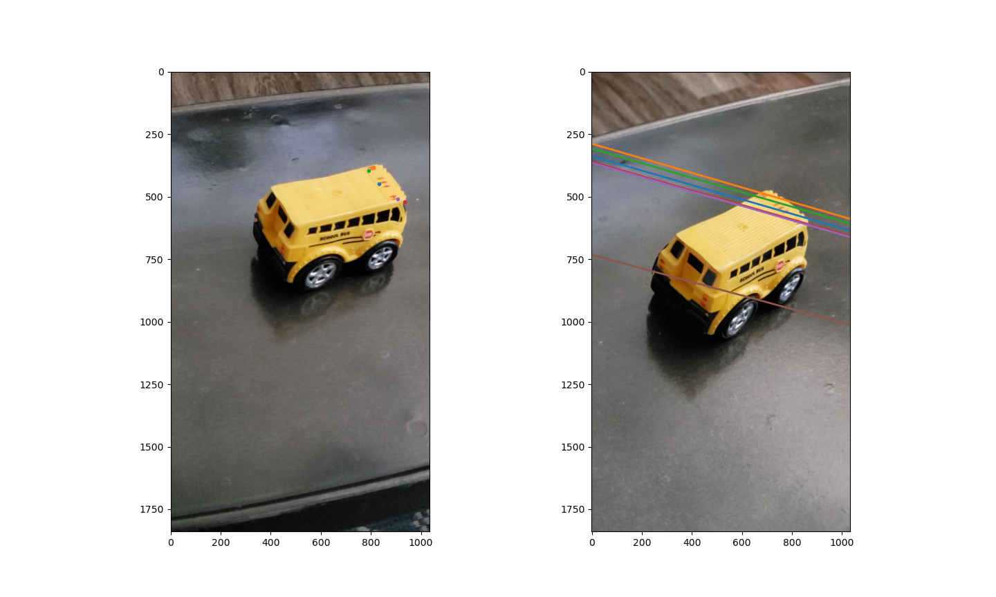
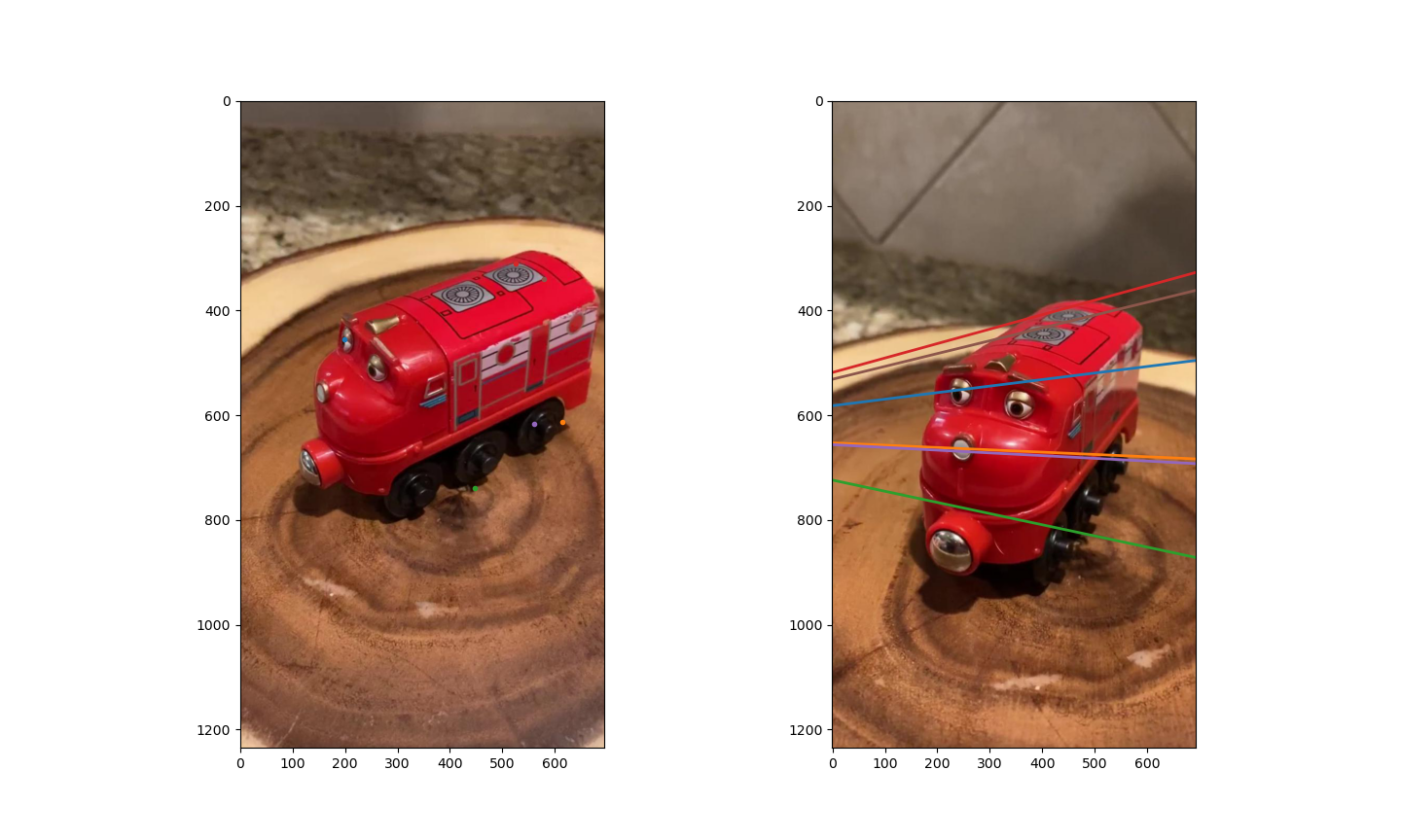
(#) Q1B 7-point Algorithm.
(##) RESULTS
(##) BRIEF IMPLEMENTATION DETAILS
1. Given the points, first step is to normalize them
2. Normalize these points using the transforamtion matrix below
T= $\begin{bmatrix}
s & 0 & -s*x_{0} \\
0 & s & -s*y_{0} \\
0 & 0 & 1
\end{bmatrix}$
3. Using these normalized coordinates, construct a matrix to recover the fundamental matrix. This can be done using the epipolar constraint $x'^{T} F x =0$
4. Using the above equation we can reduce it to the form Af = 0, where f contains all elements of the fundamental matrix and A is constructed as follows
A = $\begin{bmatrix}
x_{1}*x_{2} & x_{2}*y_{1} & x_{2} & y_{2}*x_{1} & y_{1}*y_{2} & y_{2} & x_{1} & y_{1} & 1
\end{bmatrix}$
Each point-point correspondence will give one such equation and we need 7 such equations
5. Now perform SVD and the last two eigen vectors, give us $F_{1}$ and $F_{2}$
6. We then use $F_{1}$ and $F_{2}$, to compute $\lambda$, such that
$\begin{vmatrix}
\lambda * F_{1} + (1-\lambda) * F_{2}
\end{vmatrix}$ = 0
Using the values of $F_{1}$ and $F_{2}$ we got, and $\lambda$, we can compute F = $\lambda * F_{1} + (1-\lambda) * F_{2}$
6. Once we get F, we first unnormilize the F matrix using $F_{unnormalized} = T'^{T} F_{normalized} T$ . After this, we set the last element to one and also enforce rank 2 constraint. We can do this by setting $\sigma_{3} = 0$
7. After we enforce rank 2 constraint, we again compute F by multiplying u, s and v
(#) Q2 RANSAC with 7-point and 8-point algorithm.
(#) (A) EIGHT POINT ALGORITHM
(##) RESULTS
Best $F_{chair}$ = $\begin{bmatrix}
1.81912393e-07 & 2.83125055e-06 & -1.85628366e-03\\
-3.76565087e-06 & 4.20181543e-07 & 1.39334135e-02\\
1.34857240e-03 & -1.45865225e-02 & 1.00000000e+00
\end{bmatrix}$
Best $F_{teddy}$ = $\begin{bmatrix}
4.12743758e-07 & -1.16420908e-06 & 7.46846781e-04 \\
6.04527707e-07 & 2.55973262e-07 & -3.83537574e-03 \\
-1.98508795e-03 & 3.77231096e-03 & 1.00000000e+00
\end{bmatrix}$
| Image| Epipolar plot |
| ----------- | ----------- | --- |
|Chair||
|Teddy||
(##) PLOT of Percentage of inliers vs Number of RANSAC iterations
| Image| Graph of % inliers vs # iterations |
| ----------- | ----------- | --- |
|Chair ||
|Teddy||
(##) BRIEF IMPLEMENTATION DETAILS
1. Given the points, first step is to normalize them
1a. Normalize these points using the transforamtion matrix below
T= $\begin{bmatrix}
s & 0 & -s*x_{0} \\
0 & s & -s*y_{0} \\
0 & 0 & 1
\end{bmatrix}$
2. Since the points are noisy, we select 8 random points and compute fundamental matrix using the follwing steps
3. Using these normalized coordinates, construct a matrix to recover the fundamental matrix. This can be done using the epipolar constraint $x'^{T} F x =0$
4. Using the above equation we can reduce it to the form Af = 0, where f contains all elements of the fundamental matrix and A is constructed as follows
A = $\begin{bmatrix}
x_{1}*x_{2} & x_{2}*y_{1} & x_{2} & y_{2}*x_{1} & y_{1}*y_{2} & y_{2} & x_{1} & y_{1} & 1
\end{bmatrix}$
Each point-point correspondence will give one such equation and we need 8 such equations to solve for all elements of F
Note: here I used all correspondences as suggested in the piazza post instead of using only 8 points.
5. Now perform SVD to recover all elements of F
6. Once we get F, we first unnormilize the F matrix using $F_{unnormalized} = T'^{T} F_{normalized} T$ . After this, we set the last element to one and also enforce rank 2 constraint. We can do this by setting $\sigma_{3} = 0$
7. After we enforce rank 2 constraint, we again compute F by multiplying u, s and v
8. Using this F, we then test to see if the point is an inlier or an outlier, we can do this by checking if the distance of a point from the epipolar line constructed using fundamnetal matrix < threshold
9. We check for all the point correspondences and count the number of inliers.
10. We compute F for some number of iterations where for every F, we select 8 different points and count the number of inliers.
11. We choose the F which has the highest number of inliers.
(#) (B) SEVEN POINT ALGORITHM
(##) RESULTS
Best $F_{toybus}$ = $\begin{bmatrix}
-1.70597480e-06 & 7.56283543e-06 & -5.09300085e-03 \\
-7.97290863e-06 & -1.17199023e-06 & -7.49329490e-03 \\
5.70842732e-03 & 1.06127843e-02 & 1.00000000e+00
\end{bmatrix}$
Best $F_{toytrain}$ = $\begin{bmatrix}
2.49473673e-06 & -1.14346859e-05 & 6.81372627e-03 \\
8.94709349e-06 & 3.55935955e-06 & -3.63568253e-03 \\
-7.65743983e-03 & 3.06182934e-04 & 1.00000000e+00
\end{bmatrix}$
| Image| Epipolar plot |
| ----------- | ----------- | --- |
|Toybus||
|Toytrain||
(##) PLOT of Percentage of inliers vs Number of RANSAC iterations
| Image| Graph of % inliers vs # iterations |
| ----------- | ----------- | --- |
|Toybus ||
|Toytrain||
(##) BRIEF IMPLEMENTATION DETAILS
1. Given the points, first step is to normalize them
1a. Normalize these points using the transforamtion matrix below
T= $\begin{bmatrix}
s & 0 & -s*x_{0} \\
0 & s & -s*y_{0} \\
0 & 0 & 1
\end{bmatrix}$
2. Since the points are noisy, we select 7 random points and compute fundamental matrix using the follwing steps
3. Using these normalized coordinates, construct a matrix to recover the fundamental matrix. This can be done using the epipolar constraint $x'^{T} F x =0$
4. Using the above equation we can reduce it to the form Af = 0, where f contains all elements of the fundamental matrix and A is constructed as follows
A = $\begin{bmatrix}
x_{1}*x_{2} & x_{2}*y_{1} & x_{2} & y_{2}*x_{1} & y_{1}*y_{2} & y_{2} & x_{1} & y_{1} & 1
\end{bmatrix}$
Each point-point correspondence will give one such equation and we need 7 such equations
5. Now perform SVD and the last two eigen vectors, give us $F_{1}$ and $F_{2}$
6. We then use $F_{1}$ and $F_{2}$, to compute $\lambda$, such that
$\begin{vmatrix}
\lambda * F_{1} + (1-\lambda) * F_{2}
\end{vmatrix}$ = 0
Using the values of $F_{1}$ and $F_{2}$ we got, and $\lambda$, we can compute F = $\lambda * F_{1} + (1-\lambda) * F_{2}$
6. Once we get F, we first unnormilize the F matrix using $F_{unnormalized} = T'^{T} F_{normalized} T$ . After this, we set the last element to one and also enforce rank 2 constraint. We can do this by setting $\sigma_{3} = 0$
7. After we enforce rank 2 constraint, we again compute F by multiplying u, s and v
8. Using this F, we then test to see if the point is an inlier or an outlier, we can do this by checking if the distance of a point from the epipolar line constructed using fundamnetal matrix < threshold
9. We check for all the point correspondences and count the number of inliers.
10. We compute F for some number of iterations where for every F, we select 8 different points and count the number of inliers.
11. We choose the F which has the highest number of inliers.
(##) PLOT of Number of inliers vs Number of RANSAC iterations
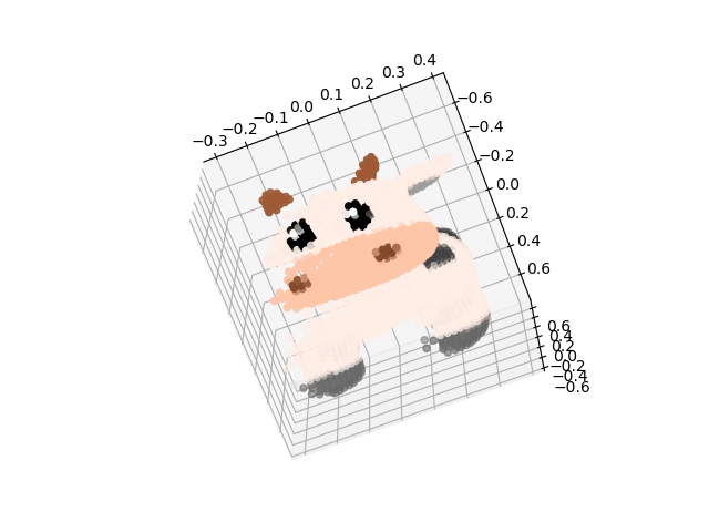
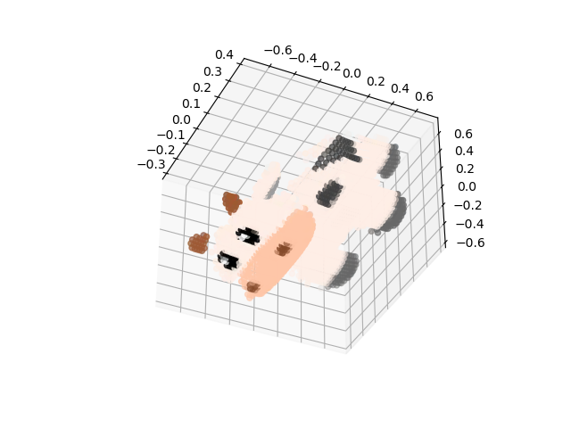
(#) Q3 TRIANGULATION.
(##) RESULTS
| Reconstruction view 1 | Reconstruction view 2 |
| ----------- | ----------- | --- |
| | |
(##) BRIEF IMPLEMENTATION DETAILS
1. Given some 2D-2D correspondences and camera projection matrices, we should construct A matrix as follows,
A= $\begin{bmatrix}
x_{1}*P_{1}^{2}-P_{1}^{0} & y_{1}*P_{1}^{2} - P_{1}^{1} & x_{2}*P_{2}^{2}-P_{2}^{0} & y_{2}*P_{2}^{2} - P_{2}^{1}
\end{bmatrix}$
2. We then compute SVD of A, and eigen vector corresponding to the last eigen vector corresponds to the points in 3D.
3. We then divide this 4D vector with the last value to get, the co-ordinates of the 3D point.
4. Plot a scatter plot to get the 3D point cloud of the object
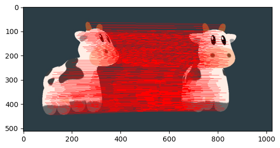
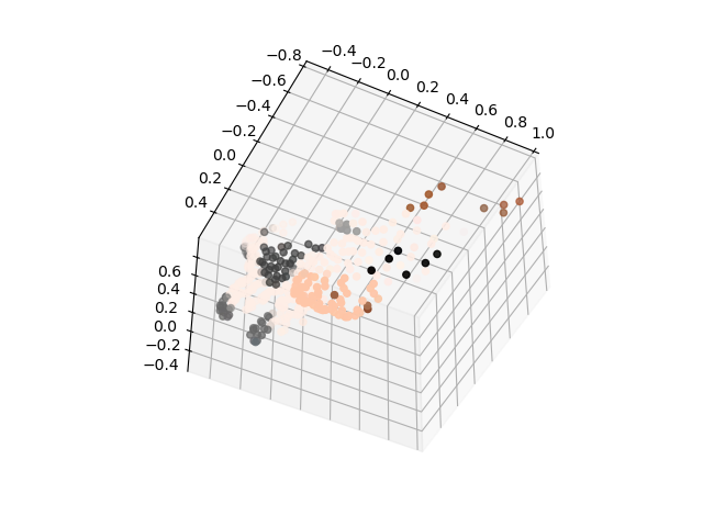
(#) Q4 Bonus 1 - Bundle Adjustment
(##) RESULTS
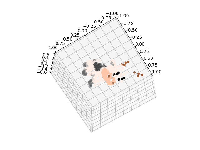
|2D Correspondences | Before Bundle Adjustment | After Bundle Adjustment |
| ----------- | ----------| ---------- |
| | |
(##) BRIEF IMPLEMENTATION DETAILS
1. Given the correpondences, we first traingulate and extend the 2D points to 3D.
2. We then reproject these points onto the image plane again and compute the reprojection error.
3. This reprojection error is the difference between the projected 3D points and the corresponding pixel co-ordinates.
4. We then use the optimize function from scipy to optimize the cameras
5. This optimized location of the points provides us with better 3D point estimates and a better reconstructed 3D point cloud
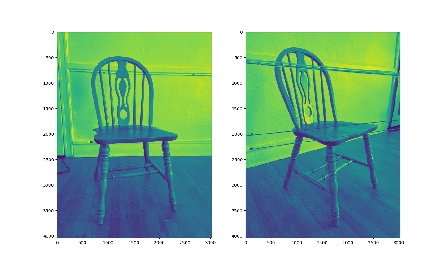
(#) Q5 Bonus 2 - Fundamental matrix estimation on your own images.
(##) RESULTS
(##) BRIEF IMPLEMENTATION DETAILS
1. First capture 2 images and then run SIFT, to get the keypoints and descriptors
2. Then use a brute force matcher called BFMatcher. This matcher gives you the matches between the two images.
3. We can use a filter to filter out bad matches and only retain the good ones.
4. These points are the point correspondences and are used to compute the fundamental matrix
5. We can then follow the steps mentioned in Q2 to get the fundamental matrix.
 (#) **DEPENDENCY INSTALLATION**
(##) Install conda environment by running
`conda create --name geometry-based-methods`
(##) To install packages
`conda install -r requirements.txt`
(#) **DEPENDENCY INSTALLATION**
(##) Install conda environment by running
`conda create --name geometry-based-methods`
(##) To install packages
`conda install -r requirements.txt`
 (##) BRIEF EXPLANATION OF IMPLEMENTATION
1. Given the points, first step is to normalize them
2. Normalize these points using the transforamtion matrix below
T= $\begin{bmatrix}
s & 0 & -s*x_{0} \\
0 & s & -s*y_{0} \\
0 & 0 & 1
\end{bmatrix}$
3. Using these normalized coordinates, construct a matrix to recover the fundamental matrix. This can be done using the epipolar constraint $x'^{T} F x =0$
4. Using the above equation we can reduce it to the form Af = 0, where f contains all elements of the fundamental matrix and A is constructed as follows
A = $\begin{bmatrix}
x_{1}*x_{2} & x_{2}*y_{1} & x_{2} & y_{2}*x_{1} & y_{1}*y_{2} & y_{2} & x_{1} & y_{1} & 1
\end{bmatrix}$
Each point-point correspondence will give one such equation and we need 8 such equations to solve for all elements of F
Note: here I used all correspondences as suggested in the piazza post instead of using only 8 points.
5. Now perform SVD to recover all elements of F
6. Once we get F, we first unnormilize the F matrix using $F_{unnormalized} = T'^{T} F_{normalized} T$ . After this, we set the last element to one and also enforce rank 2 constraint. We can do this by setting $\sigma_{3} = 0$
7. After we enforce rank 2 constraint, we again compute F by multiplying u, s and v
(#) Q1A(2).
(##) RESULTS
$E_{chair}$ = $\begin{bmatrix}
0.11320053 & 1.83773515 & 1.0941499 \\
-2.72837156 & 0.26432516 & 16.0267316 \\
-2.72725279 &-16.09946177 & 0.44957708 \\
\end{bmatrix}$
$E_{teddy}$ = $\begin{bmatrix}
0.13499427& -0.04854368& 0.79742868 \\
-0.52647433& -0.33213843& -4.66435097 \\
-1.93860455& 4.53037473& -0.02513974
\end{bmatrix}$
(##) BRIEF EXPLANATION OF IMPLEMENTATION
1. Once you compute F using 8 point algorithm, E can be estimated using the following expression, $E = K'^{T} F K$
(#) Q1B 7-point Algorithm.
(##) RESULTS
(##) BRIEF EXPLANATION OF IMPLEMENTATION
1. Given the points, first step is to normalize them
2. Normalize these points using the transforamtion matrix below
T= $\begin{bmatrix}
s & 0 & -s*x_{0} \\
0 & s & -s*y_{0} \\
0 & 0 & 1
\end{bmatrix}$
3. Using these normalized coordinates, construct a matrix to recover the fundamental matrix. This can be done using the epipolar constraint $x'^{T} F x =0$
4. Using the above equation we can reduce it to the form Af = 0, where f contains all elements of the fundamental matrix and A is constructed as follows
A = $\begin{bmatrix}
x_{1}*x_{2} & x_{2}*y_{1} & x_{2} & y_{2}*x_{1} & y_{1}*y_{2} & y_{2} & x_{1} & y_{1} & 1
\end{bmatrix}$
Each point-point correspondence will give one such equation and we need 8 such equations to solve for all elements of F
Note: here I used all correspondences as suggested in the piazza post instead of using only 8 points.
5. Now perform SVD to recover all elements of F
6. Once we get F, we first unnormilize the F matrix using $F_{unnormalized} = T'^{T} F_{normalized} T$ . After this, we set the last element to one and also enforce rank 2 constraint. We can do this by setting $\sigma_{3} = 0$
7. After we enforce rank 2 constraint, we again compute F by multiplying u, s and v
(#) Q1A(2).
(##) RESULTS
$E_{chair}$ = $\begin{bmatrix}
0.11320053 & 1.83773515 & 1.0941499 \\
-2.72837156 & 0.26432516 & 16.0267316 \\
-2.72725279 &-16.09946177 & 0.44957708 \\
\end{bmatrix}$
$E_{teddy}$ = $\begin{bmatrix}
0.13499427& -0.04854368& 0.79742868 \\
-0.52647433& -0.33213843& -4.66435097 \\
-1.93860455& 4.53037473& -0.02513974
\end{bmatrix}$
(##) BRIEF EXPLANATION OF IMPLEMENTATION
1. Once you compute F using 8 point algorithm, E can be estimated using the following expression, $E = K'^{T} F K$
(#) Q1B 7-point Algorithm.
(##) RESULTS
 (##) BRIEF IMPLEMENTATION DETAILS
1. Given the points, first step is to normalize them
2. Normalize these points using the transforamtion matrix below
T= $\begin{bmatrix}
s & 0 & -s*x_{0} \\
0 & s & -s*y_{0} \\
0 & 0 & 1
\end{bmatrix}$
3. Using these normalized coordinates, construct a matrix to recover the fundamental matrix. This can be done using the epipolar constraint $x'^{T} F x =0$
4. Using the above equation we can reduce it to the form Af = 0, where f contains all elements of the fundamental matrix and A is constructed as follows
A = $\begin{bmatrix}
x_{1}*x_{2} & x_{2}*y_{1} & x_{2} & y_{2}*x_{1} & y_{1}*y_{2} & y_{2} & x_{1} & y_{1} & 1
\end{bmatrix}$
Each point-point correspondence will give one such equation and we need 7 such equations
5. Now perform SVD and the last two eigen vectors, give us $F_{1}$ and $F_{2}$
6. We then use $F_{1}$ and $F_{2}$, to compute $\lambda$, such that
$\begin{vmatrix}
\lambda * F_{1} + (1-\lambda) * F_{2}
\end{vmatrix}$ = 0
Using the values of $F_{1}$ and $F_{2}$ we got, and $\lambda$, we can compute F = $\lambda * F_{1} + (1-\lambda) * F_{2}$
6. Once we get F, we first unnormilize the F matrix using $F_{unnormalized} = T'^{T} F_{normalized} T$ . After this, we set the last element to one and also enforce rank 2 constraint. We can do this by setting $\sigma_{3} = 0$
7. After we enforce rank 2 constraint, we again compute F by multiplying u, s and v
(#) Q2 RANSAC with 7-point and 8-point algorithm.
(#) (A) EIGHT POINT ALGORITHM
(##) RESULTS
Best $F_{chair}$ = $\begin{bmatrix}
1.81912393e-07 & 2.83125055e-06 & -1.85628366e-03\\
-3.76565087e-06 & 4.20181543e-07 & 1.39334135e-02\\
1.34857240e-03 & -1.45865225e-02 & 1.00000000e+00
\end{bmatrix}$
Best $F_{teddy}$ = $\begin{bmatrix}
4.12743758e-07 & -1.16420908e-06 & 7.46846781e-04 \\
6.04527707e-07 & 2.55973262e-07 & -3.83537574e-03 \\
-1.98508795e-03 & 3.77231096e-03 & 1.00000000e+00
\end{bmatrix}$
| Image| Epipolar plot |
| ----------- | ----------- | --- |
|Chair|
(##) BRIEF IMPLEMENTATION DETAILS
1. Given the points, first step is to normalize them
2. Normalize these points using the transforamtion matrix below
T= $\begin{bmatrix}
s & 0 & -s*x_{0} \\
0 & s & -s*y_{0} \\
0 & 0 & 1
\end{bmatrix}$
3. Using these normalized coordinates, construct a matrix to recover the fundamental matrix. This can be done using the epipolar constraint $x'^{T} F x =0$
4. Using the above equation we can reduce it to the form Af = 0, where f contains all elements of the fundamental matrix and A is constructed as follows
A = $\begin{bmatrix}
x_{1}*x_{2} & x_{2}*y_{1} & x_{2} & y_{2}*x_{1} & y_{1}*y_{2} & y_{2} & x_{1} & y_{1} & 1
\end{bmatrix}$
Each point-point correspondence will give one such equation and we need 7 such equations
5. Now perform SVD and the last two eigen vectors, give us $F_{1}$ and $F_{2}$
6. We then use $F_{1}$ and $F_{2}$, to compute $\lambda$, such that
$\begin{vmatrix}
\lambda * F_{1} + (1-\lambda) * F_{2}
\end{vmatrix}$ = 0
Using the values of $F_{1}$ and $F_{2}$ we got, and $\lambda$, we can compute F = $\lambda * F_{1} + (1-\lambda) * F_{2}$
6. Once we get F, we first unnormilize the F matrix using $F_{unnormalized} = T'^{T} F_{normalized} T$ . After this, we set the last element to one and also enforce rank 2 constraint. We can do this by setting $\sigma_{3} = 0$
7. After we enforce rank 2 constraint, we again compute F by multiplying u, s and v
(#) Q2 RANSAC with 7-point and 8-point algorithm.
(#) (A) EIGHT POINT ALGORITHM
(##) RESULTS
Best $F_{chair}$ = $\begin{bmatrix}
1.81912393e-07 & 2.83125055e-06 & -1.85628366e-03\\
-3.76565087e-06 & 4.20181543e-07 & 1.39334135e-02\\
1.34857240e-03 & -1.45865225e-02 & 1.00000000e+00
\end{bmatrix}$
Best $F_{teddy}$ = $\begin{bmatrix}
4.12743758e-07 & -1.16420908e-06 & 7.46846781e-04 \\
6.04527707e-07 & 2.55973262e-07 & -3.83537574e-03 \\
-1.98508795e-03 & 3.77231096e-03 & 1.00000000e+00
\end{bmatrix}$
| Image| Epipolar plot |
| ----------- | ----------- | --- |
|Chair|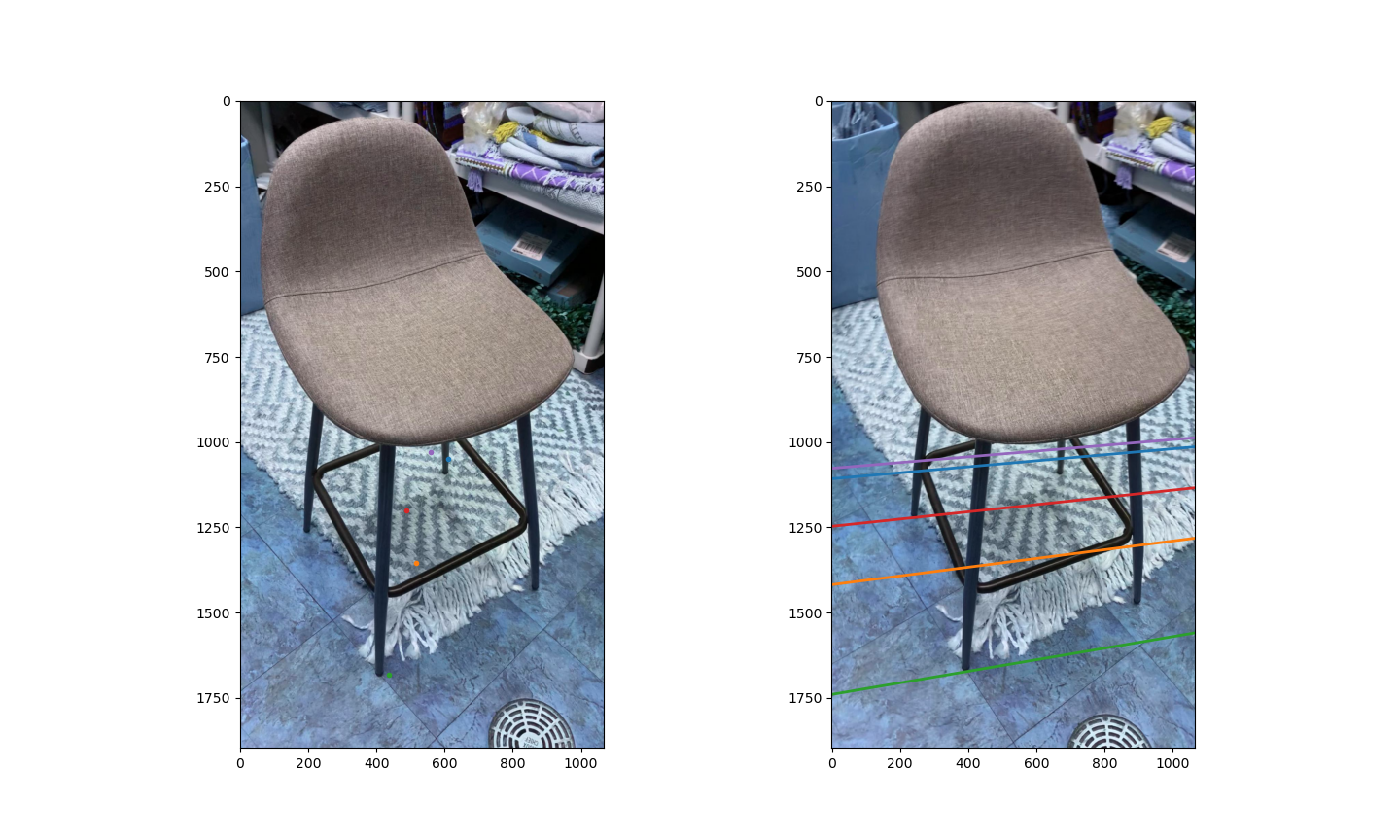 |
|Teddy|
|
|Teddy|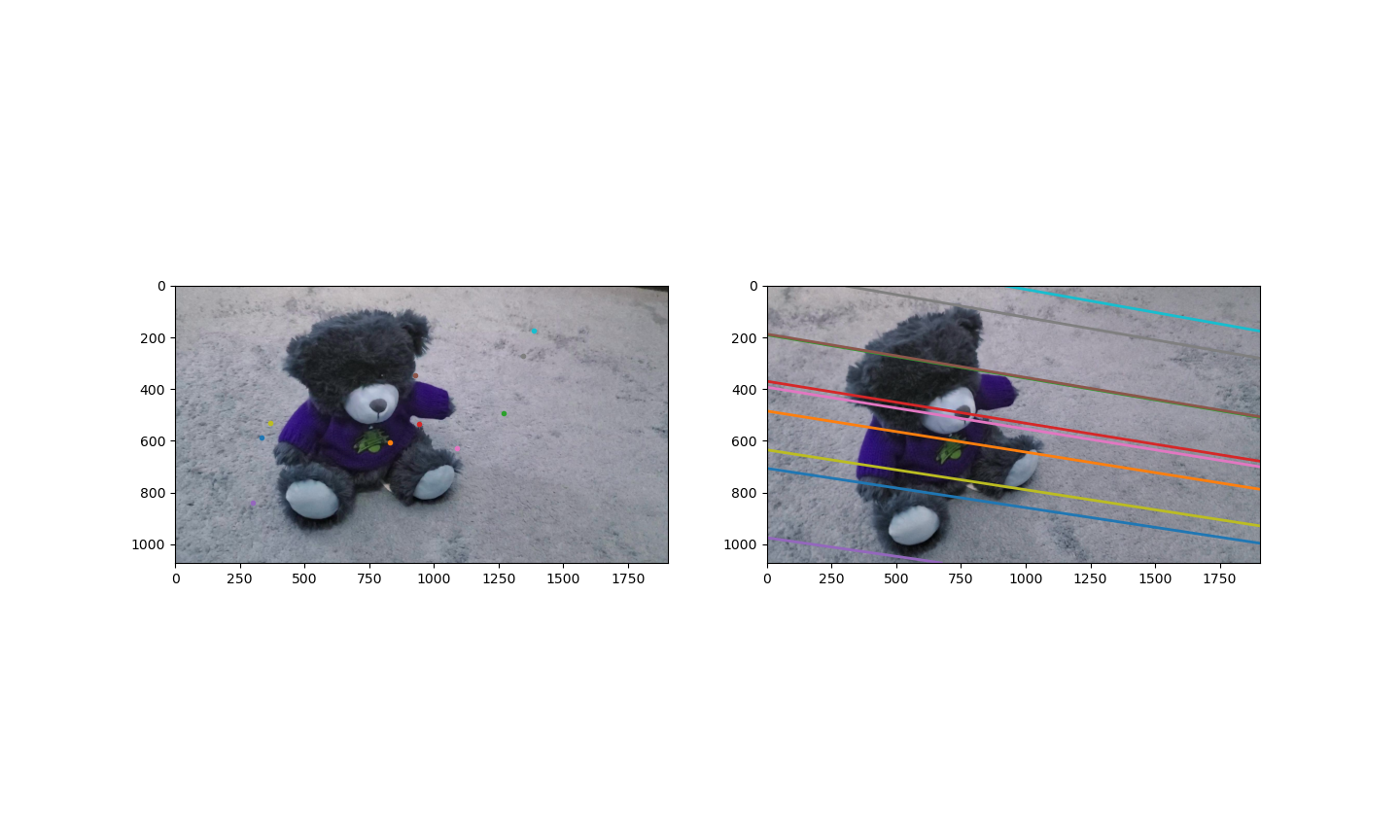 |
(##) PLOT of Percentage of inliers vs Number of RANSAC iterations
| Image| Graph of % inliers vs # iterations |
| ----------- | ----------- | --- |
|Chair |
|
(##) PLOT of Percentage of inliers vs Number of RANSAC iterations
| Image| Graph of % inliers vs # iterations |
| ----------- | ----------- | --- |
|Chair |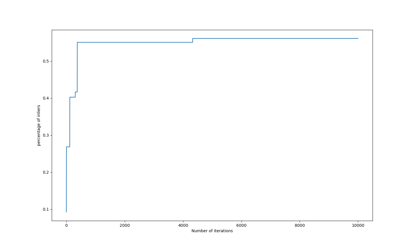 |
|Teddy|
|
|Teddy|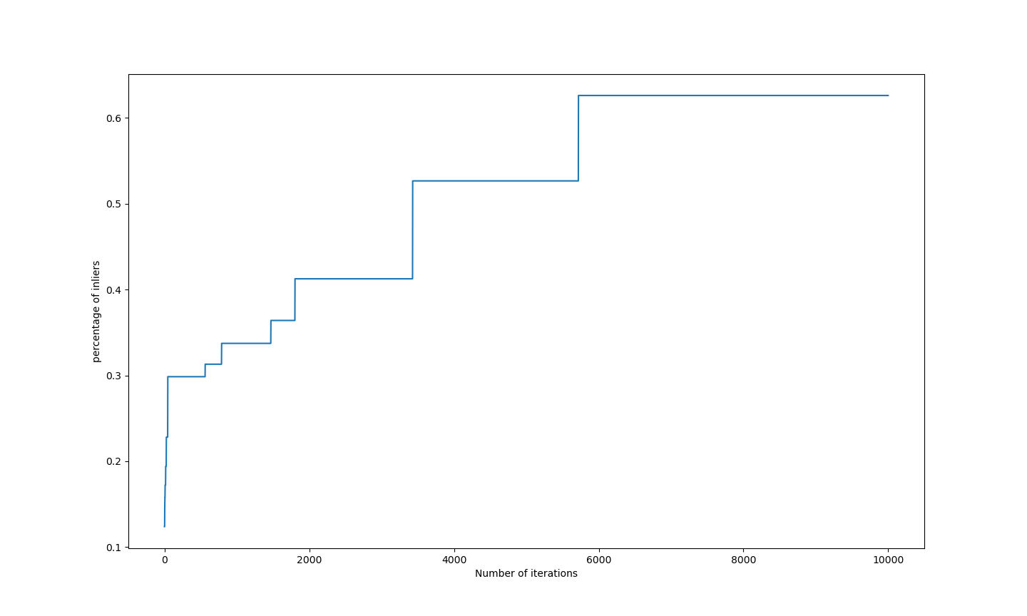 |
(##) BRIEF IMPLEMENTATION DETAILS
1. Given the points, first step is to normalize them
1a. Normalize these points using the transforamtion matrix below
T= $\begin{bmatrix}
s & 0 & -s*x_{0} \\
0 & s & -s*y_{0} \\
0 & 0 & 1
\end{bmatrix}$
2. Since the points are noisy, we select 8 random points and compute fundamental matrix using the follwing steps
3. Using these normalized coordinates, construct a matrix to recover the fundamental matrix. This can be done using the epipolar constraint $x'^{T} F x =0$
4. Using the above equation we can reduce it to the form Af = 0, where f contains all elements of the fundamental matrix and A is constructed as follows
A = $\begin{bmatrix}
x_{1}*x_{2} & x_{2}*y_{1} & x_{2} & y_{2}*x_{1} & y_{1}*y_{2} & y_{2} & x_{1} & y_{1} & 1
\end{bmatrix}$
Each point-point correspondence will give one such equation and we need 8 such equations to solve for all elements of F
Note: here I used all correspondences as suggested in the piazza post instead of using only 8 points.
5. Now perform SVD to recover all elements of F
6. Once we get F, we first unnormilize the F matrix using $F_{unnormalized} = T'^{T} F_{normalized} T$ . After this, we set the last element to one and also enforce rank 2 constraint. We can do this by setting $\sigma_{3} = 0$
7. After we enforce rank 2 constraint, we again compute F by multiplying u, s and v
8. Using this F, we then test to see if the point is an inlier or an outlier, we can do this by checking if the distance of a point from the epipolar line constructed using fundamnetal matrix < threshold
9. We check for all the point correspondences and count the number of inliers.
10. We compute F for some number of iterations where for every F, we select 8 different points and count the number of inliers.
11. We choose the F which has the highest number of inliers.
(#) (B) SEVEN POINT ALGORITHM
(##) RESULTS
Best $F_{toybus}$ = $\begin{bmatrix}
-1.70597480e-06 & 7.56283543e-06 & -5.09300085e-03 \\
-7.97290863e-06 & -1.17199023e-06 & -7.49329490e-03 \\
5.70842732e-03 & 1.06127843e-02 & 1.00000000e+00
\end{bmatrix}$
Best $F_{toytrain}$ = $\begin{bmatrix}
2.49473673e-06 & -1.14346859e-05 & 6.81372627e-03 \\
8.94709349e-06 & 3.55935955e-06 & -3.63568253e-03 \\
-7.65743983e-03 & 3.06182934e-04 & 1.00000000e+00
\end{bmatrix}$
| Image| Epipolar plot |
| ----------- | ----------- | --- |
|Toybus|
|
(##) BRIEF IMPLEMENTATION DETAILS
1. Given the points, first step is to normalize them
1a. Normalize these points using the transforamtion matrix below
T= $\begin{bmatrix}
s & 0 & -s*x_{0} \\
0 & s & -s*y_{0} \\
0 & 0 & 1
\end{bmatrix}$
2. Since the points are noisy, we select 8 random points and compute fundamental matrix using the follwing steps
3. Using these normalized coordinates, construct a matrix to recover the fundamental matrix. This can be done using the epipolar constraint $x'^{T} F x =0$
4. Using the above equation we can reduce it to the form Af = 0, where f contains all elements of the fundamental matrix and A is constructed as follows
A = $\begin{bmatrix}
x_{1}*x_{2} & x_{2}*y_{1} & x_{2} & y_{2}*x_{1} & y_{1}*y_{2} & y_{2} & x_{1} & y_{1} & 1
\end{bmatrix}$
Each point-point correspondence will give one such equation and we need 8 such equations to solve for all elements of F
Note: here I used all correspondences as suggested in the piazza post instead of using only 8 points.
5. Now perform SVD to recover all elements of F
6. Once we get F, we first unnormilize the F matrix using $F_{unnormalized} = T'^{T} F_{normalized} T$ . After this, we set the last element to one and also enforce rank 2 constraint. We can do this by setting $\sigma_{3} = 0$
7. After we enforce rank 2 constraint, we again compute F by multiplying u, s and v
8. Using this F, we then test to see if the point is an inlier or an outlier, we can do this by checking if the distance of a point from the epipolar line constructed using fundamnetal matrix < threshold
9. We check for all the point correspondences and count the number of inliers.
10. We compute F for some number of iterations where for every F, we select 8 different points and count the number of inliers.
11. We choose the F which has the highest number of inliers.
(#) (B) SEVEN POINT ALGORITHM
(##) RESULTS
Best $F_{toybus}$ = $\begin{bmatrix}
-1.70597480e-06 & 7.56283543e-06 & -5.09300085e-03 \\
-7.97290863e-06 & -1.17199023e-06 & -7.49329490e-03 \\
5.70842732e-03 & 1.06127843e-02 & 1.00000000e+00
\end{bmatrix}$
Best $F_{toytrain}$ = $\begin{bmatrix}
2.49473673e-06 & -1.14346859e-05 & 6.81372627e-03 \\
8.94709349e-06 & 3.55935955e-06 & -3.63568253e-03 \\
-7.65743983e-03 & 3.06182934e-04 & 1.00000000e+00
\end{bmatrix}$
| Image| Epipolar plot |
| ----------- | ----------- | --- |
|Toybus|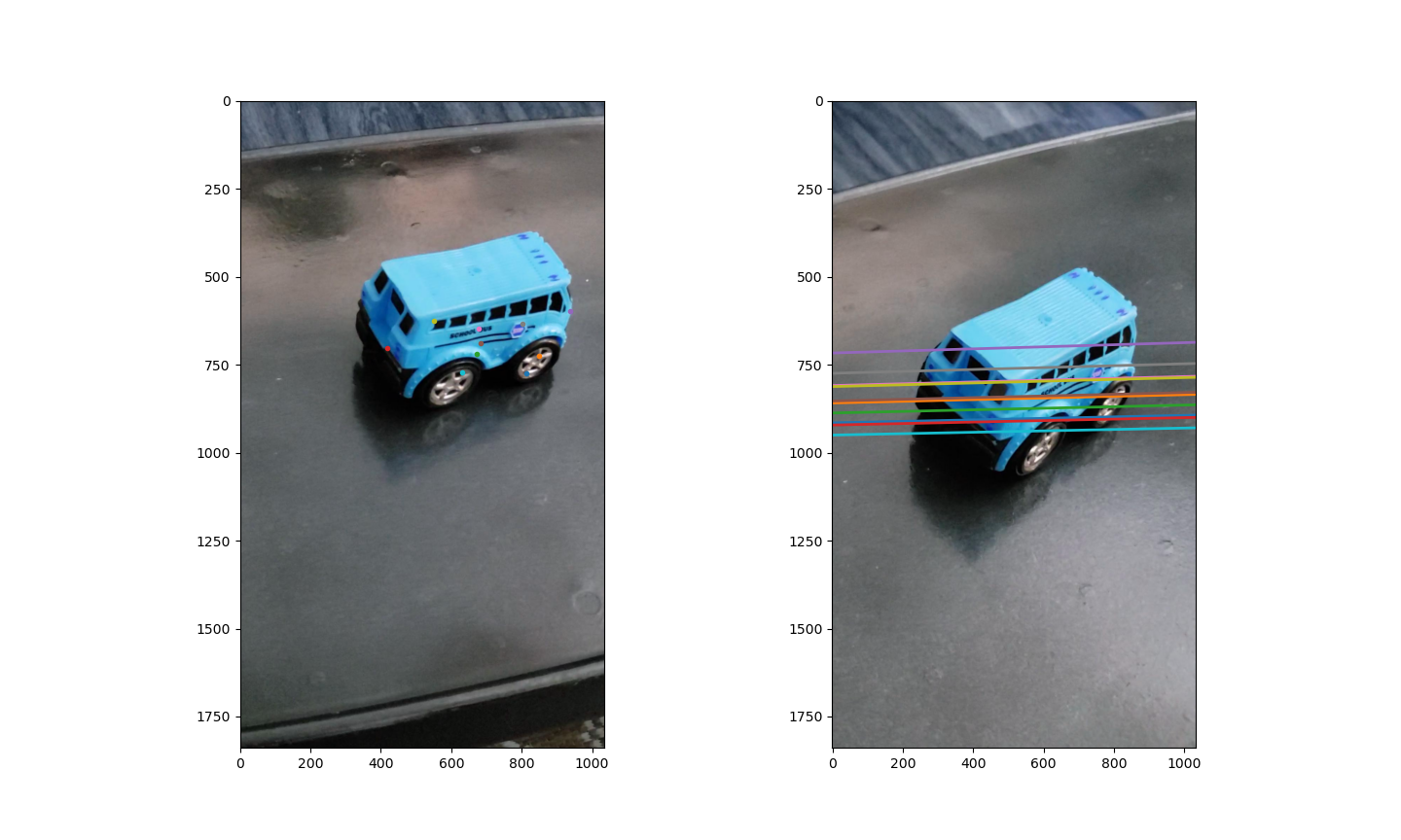 |
|Toytrain|
|
|Toytrain|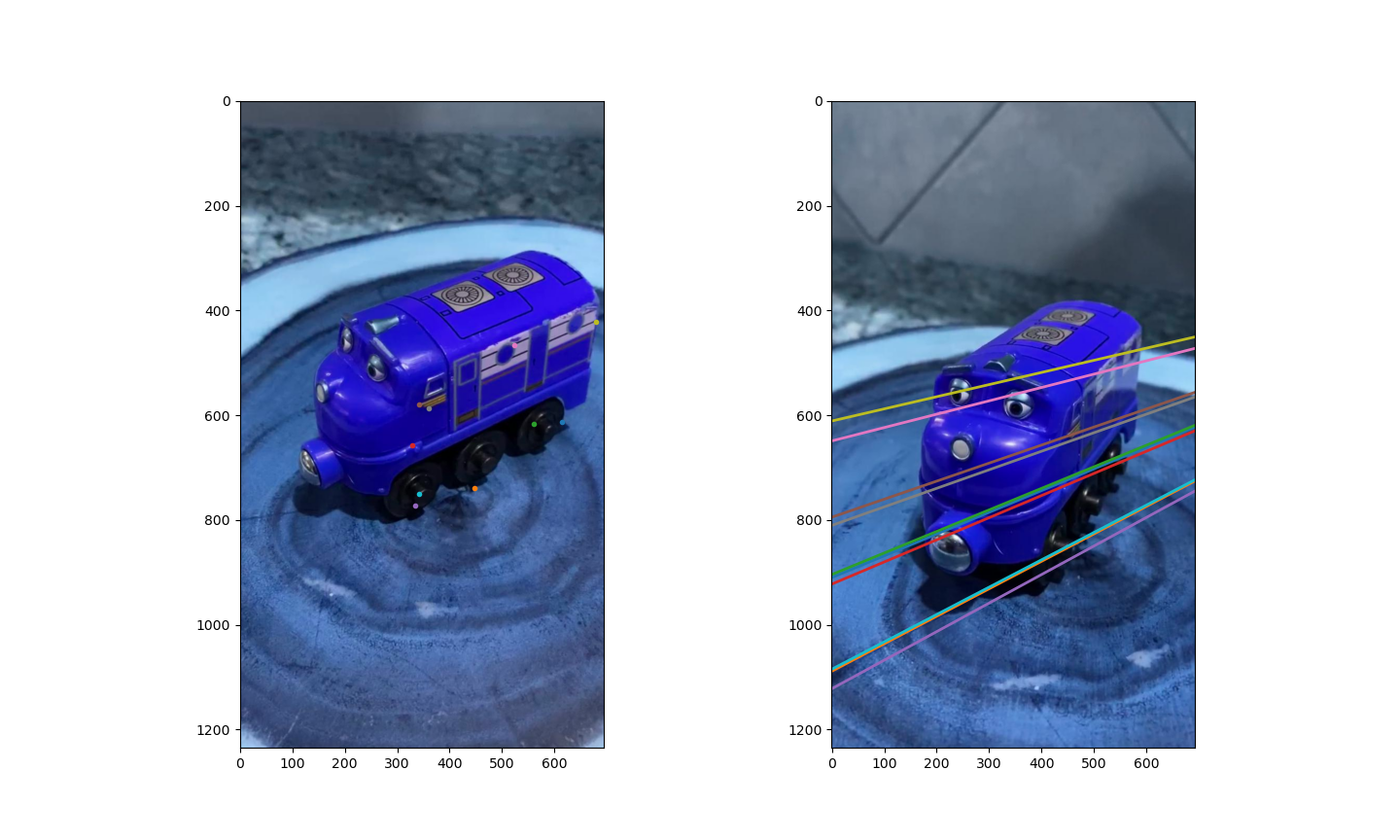 |
(##) PLOT of Percentage of inliers vs Number of RANSAC iterations
| Image| Graph of % inliers vs # iterations |
| ----------- | ----------- | --- |
|Toybus |
|
(##) PLOT of Percentage of inliers vs Number of RANSAC iterations
| Image| Graph of % inliers vs # iterations |
| ----------- | ----------- | --- |
|Toybus |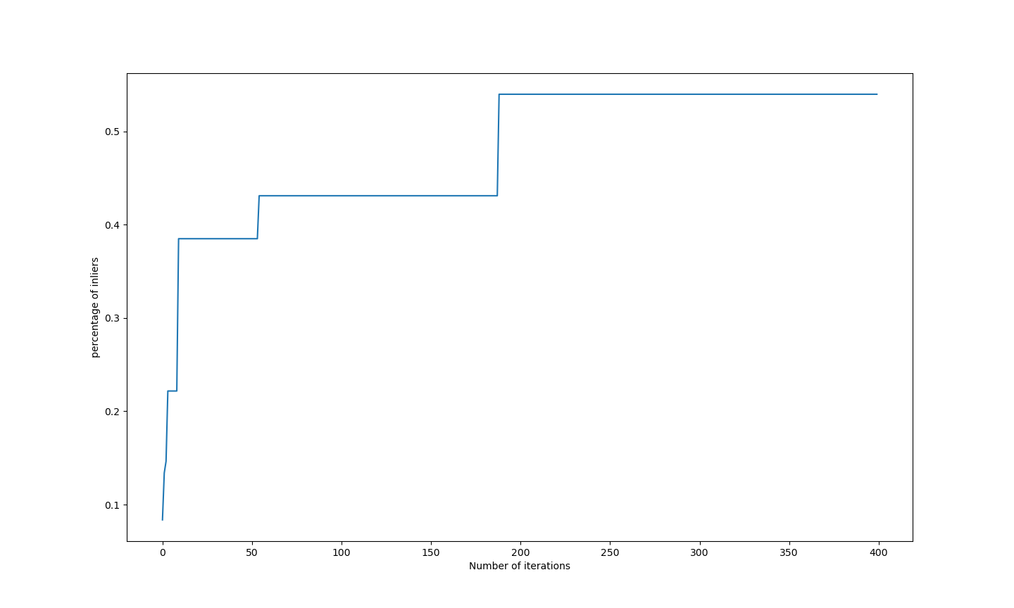 |
|Toytrain|
|
|Toytrain|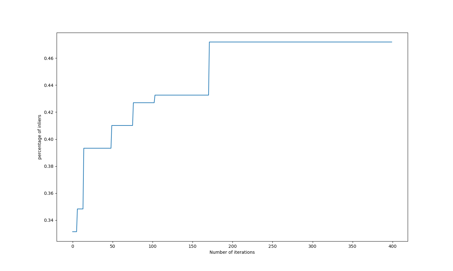 |
(##) BRIEF IMPLEMENTATION DETAILS
1. Given the points, first step is to normalize them
1a. Normalize these points using the transforamtion matrix below
T= $\begin{bmatrix}
s & 0 & -s*x_{0} \\
0 & s & -s*y_{0} \\
0 & 0 & 1
\end{bmatrix}$
2. Since the points are noisy, we select 7 random points and compute fundamental matrix using the follwing steps
3. Using these normalized coordinates, construct a matrix to recover the fundamental matrix. This can be done using the epipolar constraint $x'^{T} F x =0$
4. Using the above equation we can reduce it to the form Af = 0, where f contains all elements of the fundamental matrix and A is constructed as follows
A = $\begin{bmatrix}
x_{1}*x_{2} & x_{2}*y_{1} & x_{2} & y_{2}*x_{1} & y_{1}*y_{2} & y_{2} & x_{1} & y_{1} & 1
\end{bmatrix}$
Each point-point correspondence will give one such equation and we need 7 such equations
5. Now perform SVD and the last two eigen vectors, give us $F_{1}$ and $F_{2}$
6. We then use $F_{1}$ and $F_{2}$, to compute $\lambda$, such that
$\begin{vmatrix}
\lambda * F_{1} + (1-\lambda) * F_{2}
\end{vmatrix}$ = 0
Using the values of $F_{1}$ and $F_{2}$ we got, and $\lambda$, we can compute F = $\lambda * F_{1} + (1-\lambda) * F_{2}$
6. Once we get F, we first unnormilize the F matrix using $F_{unnormalized} = T'^{T} F_{normalized} T$ . After this, we set the last element to one and also enforce rank 2 constraint. We can do this by setting $\sigma_{3} = 0$
7. After we enforce rank 2 constraint, we again compute F by multiplying u, s and v
8. Using this F, we then test to see if the point is an inlier or an outlier, we can do this by checking if the distance of a point from the epipolar line constructed using fundamnetal matrix < threshold
9. We check for all the point correspondences and count the number of inliers.
10. We compute F for some number of iterations where for every F, we select 8 different points and count the number of inliers.
11. We choose the F which has the highest number of inliers.
(##) PLOT of Number of inliers vs Number of RANSAC iterations
(#) Q3 TRIANGULATION.
(##) RESULTS
| Reconstruction view 1 | Reconstruction view 2 |
| ----------- | ----------- | --- |
|
|
(##) BRIEF IMPLEMENTATION DETAILS
1. Given the points, first step is to normalize them
1a. Normalize these points using the transforamtion matrix below
T= $\begin{bmatrix}
s & 0 & -s*x_{0} \\
0 & s & -s*y_{0} \\
0 & 0 & 1
\end{bmatrix}$
2. Since the points are noisy, we select 7 random points and compute fundamental matrix using the follwing steps
3. Using these normalized coordinates, construct a matrix to recover the fundamental matrix. This can be done using the epipolar constraint $x'^{T} F x =0$
4. Using the above equation we can reduce it to the form Af = 0, where f contains all elements of the fundamental matrix and A is constructed as follows
A = $\begin{bmatrix}
x_{1}*x_{2} & x_{2}*y_{1} & x_{2} & y_{2}*x_{1} & y_{1}*y_{2} & y_{2} & x_{1} & y_{1} & 1
\end{bmatrix}$
Each point-point correspondence will give one such equation and we need 7 such equations
5. Now perform SVD and the last two eigen vectors, give us $F_{1}$ and $F_{2}$
6. We then use $F_{1}$ and $F_{2}$, to compute $\lambda$, such that
$\begin{vmatrix}
\lambda * F_{1} + (1-\lambda) * F_{2}
\end{vmatrix}$ = 0
Using the values of $F_{1}$ and $F_{2}$ we got, and $\lambda$, we can compute F = $\lambda * F_{1} + (1-\lambda) * F_{2}$
6. Once we get F, we first unnormilize the F matrix using $F_{unnormalized} = T'^{T} F_{normalized} T$ . After this, we set the last element to one and also enforce rank 2 constraint. We can do this by setting $\sigma_{3} = 0$
7. After we enforce rank 2 constraint, we again compute F by multiplying u, s and v
8. Using this F, we then test to see if the point is an inlier or an outlier, we can do this by checking if the distance of a point from the epipolar line constructed using fundamnetal matrix < threshold
9. We check for all the point correspondences and count the number of inliers.
10. We compute F for some number of iterations where for every F, we select 8 different points and count the number of inliers.
11. We choose the F which has the highest number of inliers.
(##) PLOT of Number of inliers vs Number of RANSAC iterations
(#) Q3 TRIANGULATION.
(##) RESULTS
| Reconstruction view 1 | Reconstruction view 2 |
| ----------- | ----------- | --- |
|  |
|  |
(##) BRIEF IMPLEMENTATION DETAILS
1. Given some 2D-2D correspondences and camera projection matrices, we should construct A matrix as follows,
A= $\begin{bmatrix}
x_{1}*P_{1}^{2}-P_{1}^{0} & y_{1}*P_{1}^{2} - P_{1}^{1} & x_{2}*P_{2}^{2}-P_{2}^{0} & y_{2}*P_{2}^{2} - P_{2}^{1}
\end{bmatrix}$
2. We then compute SVD of A, and eigen vector corresponding to the last eigen vector corresponds to the points in 3D.
3. We then divide this 4D vector with the last value to get, the co-ordinates of the 3D point.
4. Plot a scatter plot to get the 3D point cloud of the object
(#) Q4 Bonus 1 - Bundle Adjustment
(##) RESULTS
|2D Correspondences | Before Bundle Adjustment | After Bundle Adjustment |
| ----------- | ----------| ---------- |
|
|
(##) BRIEF IMPLEMENTATION DETAILS
1. Given some 2D-2D correspondences and camera projection matrices, we should construct A matrix as follows,
A= $\begin{bmatrix}
x_{1}*P_{1}^{2}-P_{1}^{0} & y_{1}*P_{1}^{2} - P_{1}^{1} & x_{2}*P_{2}^{2}-P_{2}^{0} & y_{2}*P_{2}^{2} - P_{2}^{1}
\end{bmatrix}$
2. We then compute SVD of A, and eigen vector corresponding to the last eigen vector corresponds to the points in 3D.
3. We then divide this 4D vector with the last value to get, the co-ordinates of the 3D point.
4. Plot a scatter plot to get the 3D point cloud of the object
(#) Q4 Bonus 1 - Bundle Adjustment
(##) RESULTS
|2D Correspondences | Before Bundle Adjustment | After Bundle Adjustment |
| ----------- | ----------| ---------- |
| |
|  |
|  (##) BRIEF IMPLEMENTATION DETAILS
1. Given the correpondences, we first traingulate and extend the 2D points to 3D.
2. We then reproject these points onto the image plane again and compute the reprojection error.
3. This reprojection error is the difference between the projected 3D points and the corresponding pixel co-ordinates.
4. We then use the optimize function from scipy to optimize the cameras
5. This optimized location of the points provides us with better 3D point estimates and a better reconstructed 3D point cloud
(#) Q5 Bonus 2 - Fundamental matrix estimation on your own images.
(##) RESULTS
(##) BRIEF IMPLEMENTATION DETAILS
1. Given the correpondences, we first traingulate and extend the 2D points to 3D.
2. We then reproject these points onto the image plane again and compute the reprojection error.
3. This reprojection error is the difference between the projected 3D points and the corresponding pixel co-ordinates.
4. We then use the optimize function from scipy to optimize the cameras
5. This optimized location of the points provides us with better 3D point estimates and a better reconstructed 3D point cloud
(#) Q5 Bonus 2 - Fundamental matrix estimation on your own images.
(##) RESULTS
 (##) BRIEF IMPLEMENTATION DETAILS
1. First capture 2 images and then run SIFT, to get the keypoints and descriptors
2. Then use a brute force matcher called BFMatcher. This matcher gives you the matches between the two images.
3. We can use a filter to filter out bad matches and only retain the good ones.
4. These points are the point correspondences and are used to compute the fundamental matrix
5. We can then follow the steps mentioned in Q2 to get the fundamental matrix.
(##) BRIEF IMPLEMENTATION DETAILS
1. First capture 2 images and then run SIFT, to get the keypoints and descriptors
2. Then use a brute force matcher called BFMatcher. This matcher gives you the matches between the two images.
3. We can use a filter to filter out bad matches and only retain the good ones.
4. These points are the point correspondences and are used to compute the fundamental matrix
5. We can then follow the steps mentioned in Q2 to get the fundamental matrix.