**Assignment 2: Single View Reconstruction**
Student name: Abhishek Pavani
(##) LATE DAYS : 0
(#) **DEPENDENCY INSTALLATION**
(##) Install conda environment by running
`conda create --name geometry-based-methods`
(##) To install packages
`conda install -r requirements.txt`
(#) **RUN CODE**
(##) To construct point correspondences, use the following command
`python point_correspondences.py`
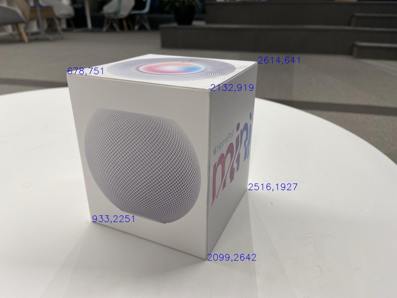
Note: Once you run the above command, an image opens up and then you can mark 6 points on the cube. As soon as you mark 6 points, a 'points_1b.npz' file will get created and an image with the name 'annotated_cuboid.jpg' will get saved
Note: For ease of use, the correspondences have already been saved. Select the appropriate question number in all of the commands below
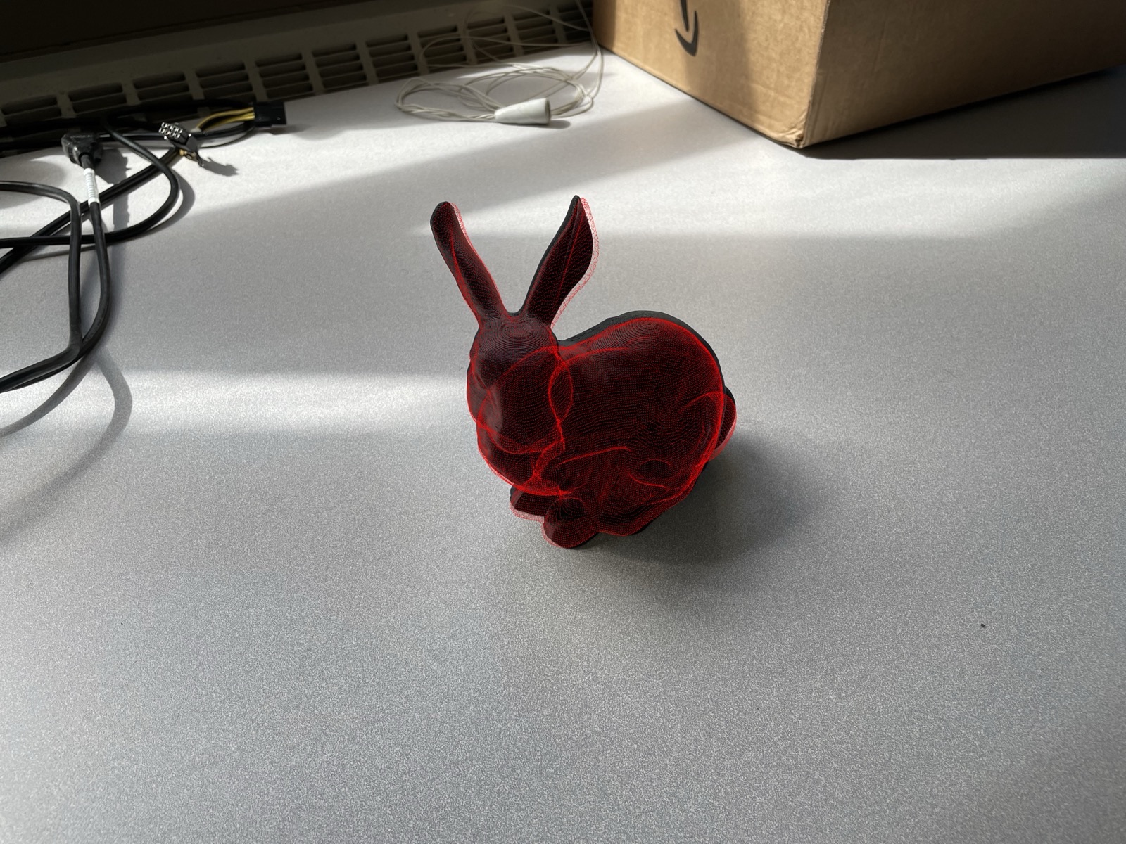
(##) To run code for Q1(a) and see the projected points on bunny, run
`python main.py --question='q1a'`
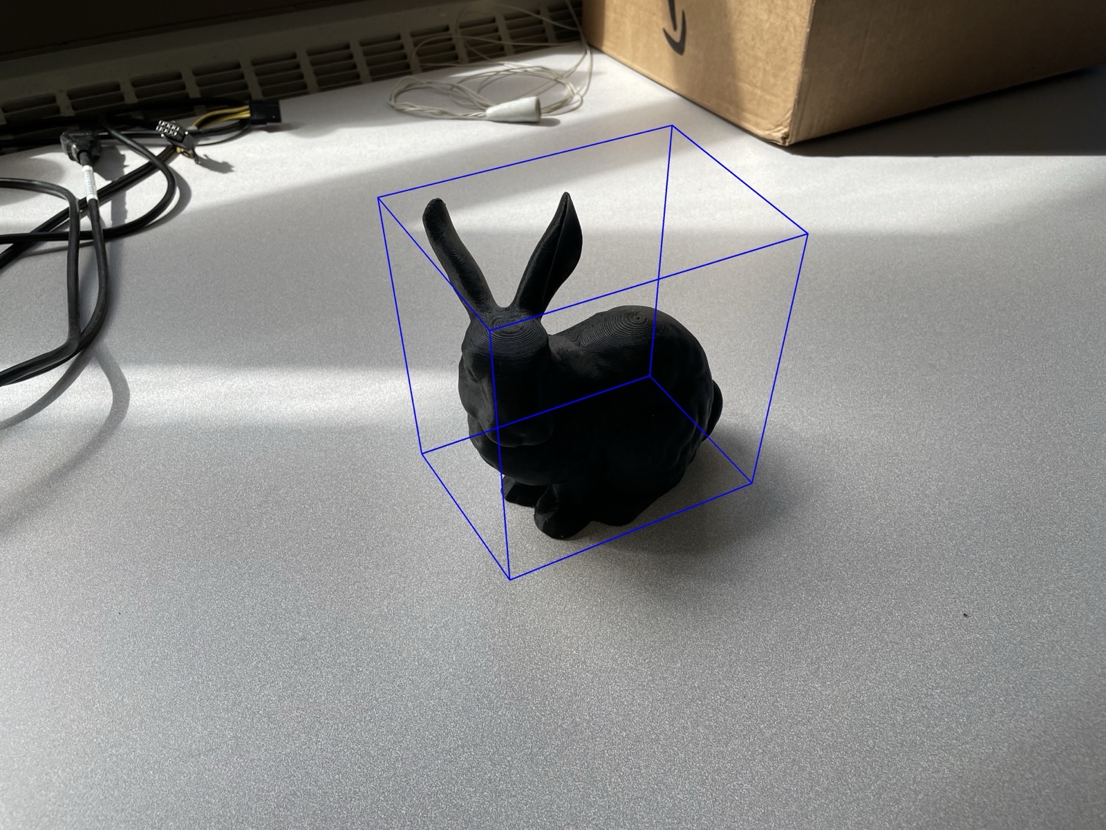
(##) To see the bounding box around the bunny, run
`python main.py --question='q1a_bb'`
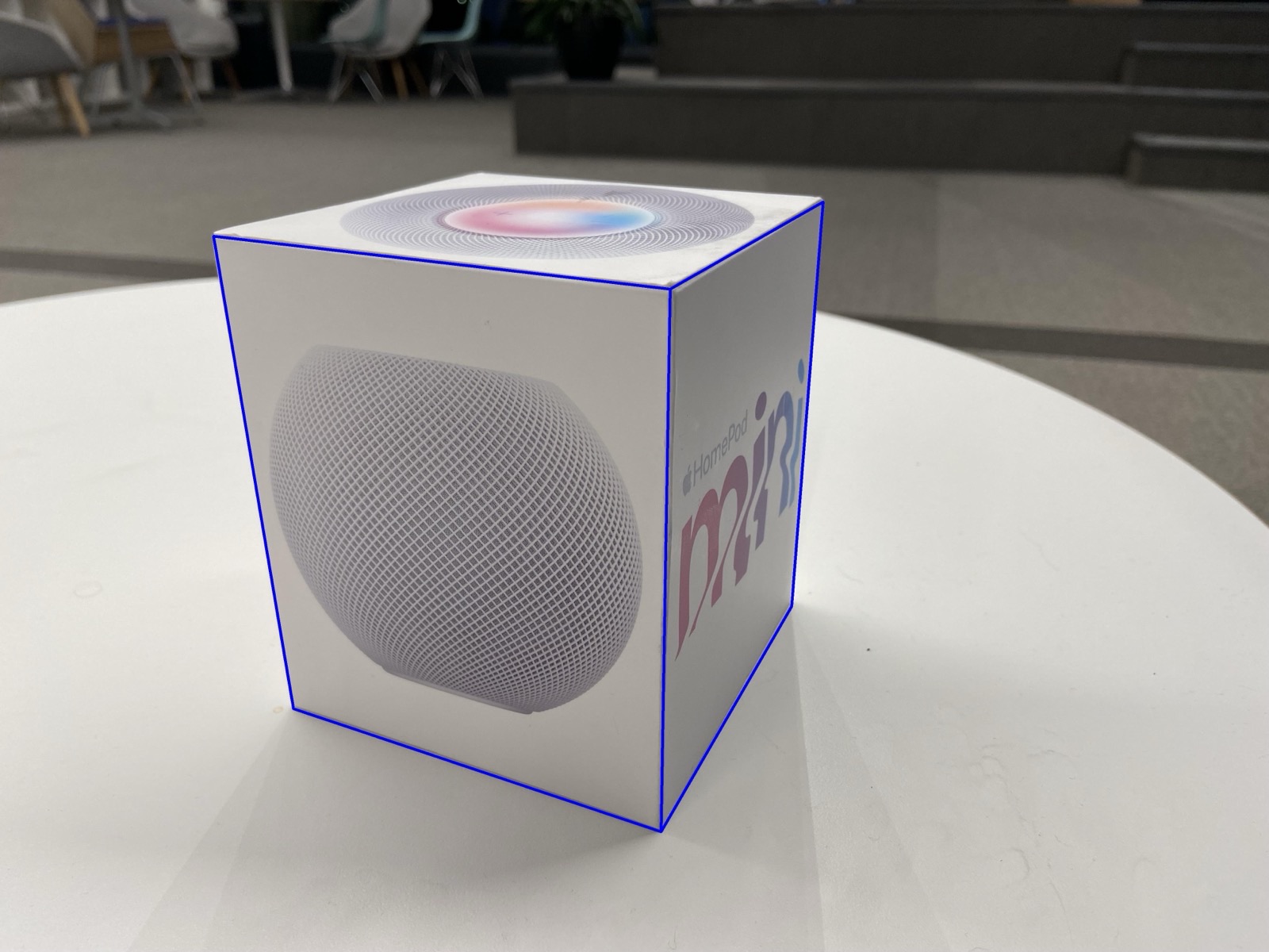
(##) To see the bounding box around the cube for Q1(b), run
`python main.py --question='q1b'`
(##) To plot the image center and the lines connecting the three vanishing points and get the computed intrinsic matrix K, run
`python main.py --question='q2a'`
(##) To compute intrinsic matrix K, run
`python main.py --question='q2a'`
(##) To compute intrinsic matrix and camera center for question 2b,run
`python main.py --question='q2b'`
(##) To compute intrinsic matrix and camera center for question 2b,run
`python main.py --question='q2c'`
(##) To get the single-view reconstruction of the given image, run
`python main.py --question='q3a'`
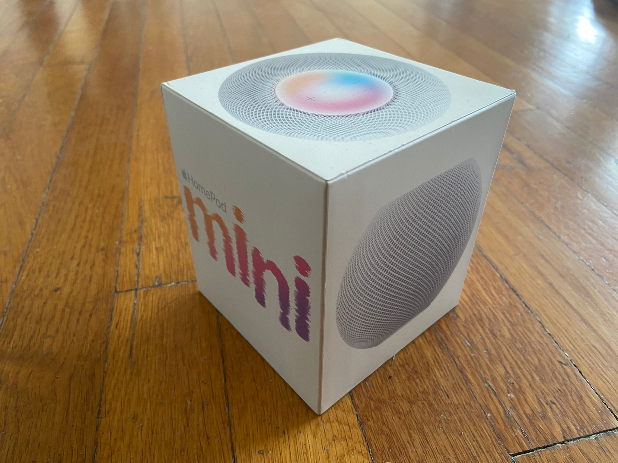
(##) To run single view reconstruction of other images, run,
`python main.py --question='q3b' --image_path='data/ec2/homepod.jpeg' --coordinate_path='coordinates/homepod.npz'`
(#) Q1a.
(##) RESULTS
Camera Projection Matrix P =
[[ 6.36808707e+03 -2.94538221e+03 1.11960341e+03 2.22627325e+03]
[-9.76912656e+02 -6.75979592e+03 2.02015897e+03 1.82252030e+03]
[ 5.50350274e-01 -1.42297625e+00 -7.51628034e-01 1.00000000e+00]]
(#) Q1b.
(##) RESULTS
Camera Projection Matrix P =
[[ 8.00714922e+00 -3.07780813e+00 1.09825917e+01 9.32661152e+02]
[-4.05170890e-03 -1.31564082e+01 2.69162932e-01 2.25105340e+03]
[-1.38455973e-03 -1.53868687e-03 3.06680140e-03 1.00000000e+00]]
| Input Image | Annotated 2D points |Example Result |
| ----------- | ----------- | ------- |
| | | |
(#) Q2a.
(##) RESULTS
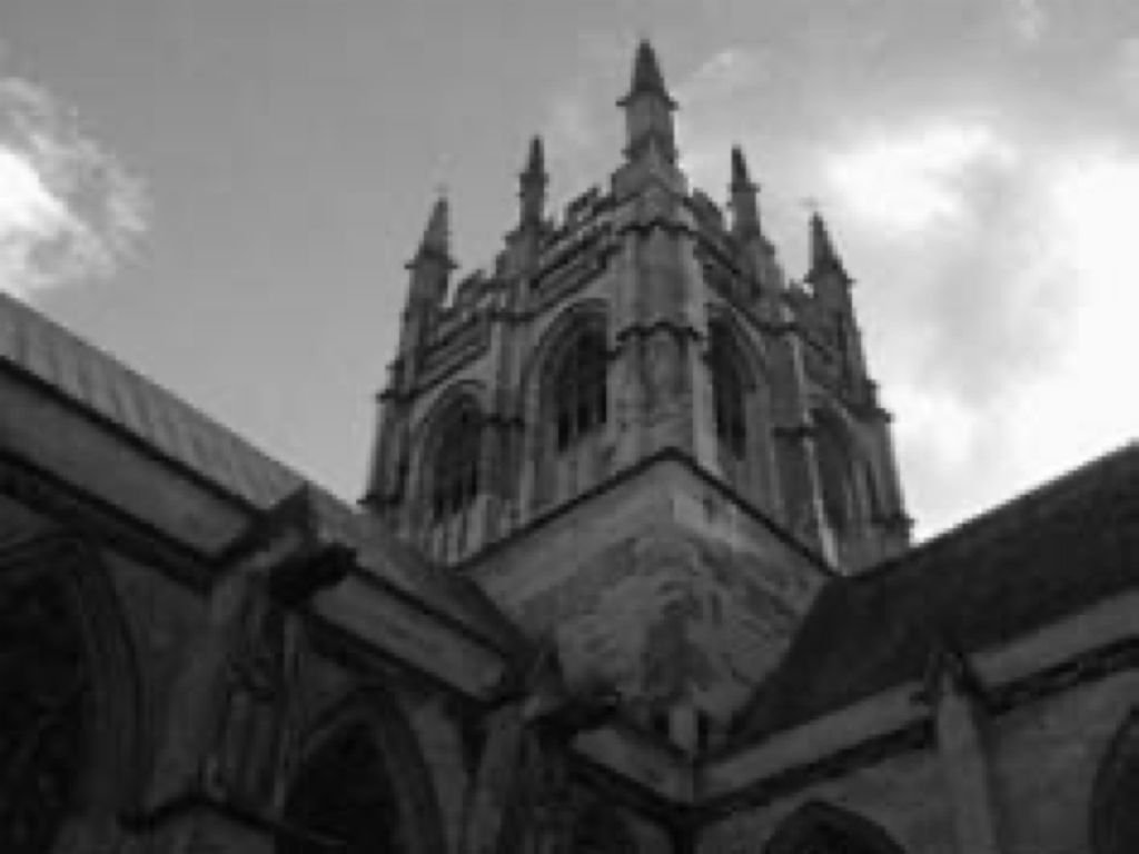
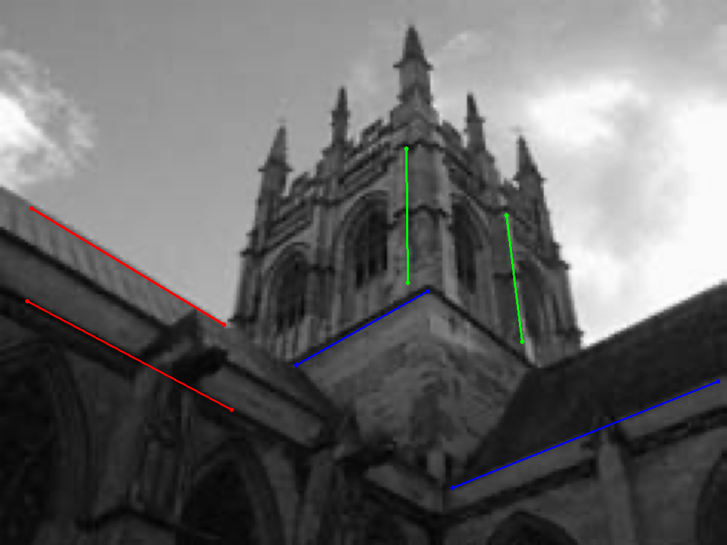
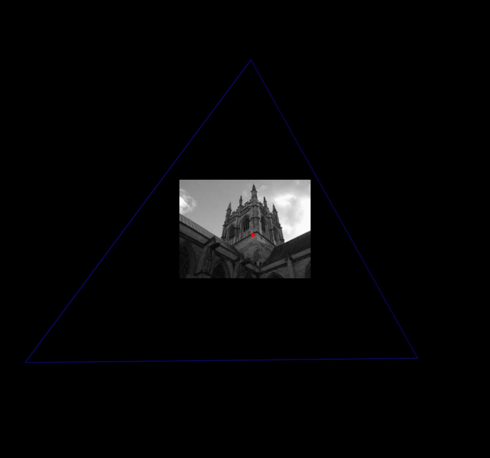
| Input Image | Annotated Parallel Lines | Vanishing points and principal point |
| ----------- | ----------- | ----------- |
| | | |
(##) BRIEF IMPLEMENTATION DETAILS
1. Draw 3 sets of parallel lines which are orthogonal to each other or use use the annotations provided.
2. Compute the vanishing points of these lines by taking the cross product between parallel lines
3. Compute the vanishing line by taking cross product between 2 vanishing points. Since we have 3 vanishing points, we can create 3 vanishing lines which all form a triangle.
4. The prinicpal point can then be found out by computing the orthocenter of the triangle
5. Since the pixels are square, we can compute the focal length by applying simple geometric formulae.
6. Intrinsic matrix K obtained by this process is reported below
K= $\begin{bmatrix}
1.15357143e+03 & 0 & 574 \\
0 & 1.15357143e+03 & 431 \\
0 & 0 & 1
\end{bmatrix}$
7. Principal point is (574, 431)
(#) Q2b.
(##) RESULTS
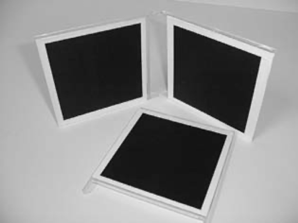
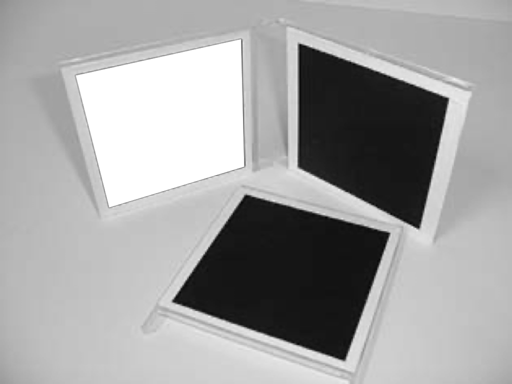
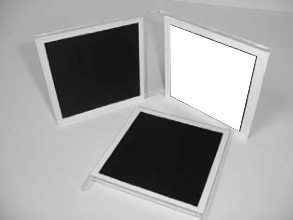
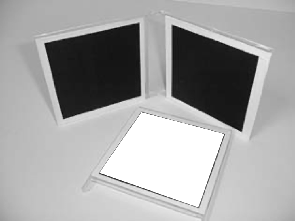
| Input Image | Annotated Square 1 | Annotated Square 2 | Annotated Square 3 |
| ----------- | ----------- | ----------- | ----------- | ----- |
| | | | |
| Angle Between planes |
| ----------- | ------|
|Plane 1 and 2: 67.47032019654877|
|Plane 2 and 3: 94.80530541410337|
|Plane 1 and 3: 92.22151037775696|
Intrinsic Matrix:
K= $\begin{bmatrix}
1.08400790e+03 & -1.13937390e+01 & 5.15917724e+02 \\
0 & 1.07775639e+03 & 3.95113033e+02 \\
0 & 0 & 1
\end{bmatrix}$
(##) BRIEF IMPLEMENTATION DETAILS
1. For this question, first compute the homography between the metrically rectified space and image space.
We can use the constraints,
${h_{1}}^T$ $\omega$ $h_{2}$ = 0
${h_{1}}^T$ $\omega$ $h_{1}$ = ${h_{2}}^T$ $\omega$ $h_{2}$
2. Each square will give us two constraints and we will finally have an A matrix which will be 6x6 and we have 6 unknowns in the $\omega$ matrix
3. We can then use SVD to get the 6 values of the $\omega$ matrix
4. Use cholesky decomposition to get K.
5. To compute the angle between the planes, first find normals to the plane. This can be done by first computing the vanshing points and then we can compute the direction of the ray by using
$d_{1}$ = $K^{-1}$ $v_{1}$
$d_{2}$ = $K^{-1}$ $v_{2}$
6. We then compute the cross product between the directions to get the normal to the planes
7. After this take the dot product between the plane normals to get the angles between the planes
(#) Q2c.
(##) RESULTS
| Input Image | Annotations|
| ----------- | ----------- | ------- |
| | |
| Angle Between planes |
| ----------- | ------|
|Plane 1 and 2: 62.67616513786972|
|Plane 2 and 3: 59.59931039190723|
|Plane 1 and 3: 92.6447856315416|
Intrinsic Matrix:
K= $\begin{bmatrix}
1.66636154e+03 & -7.86141939e+01 & 9.97116245e+02 \\
0 & 1.15357143e+03 & 5.11778464e+02 \\
0 & 0 & 1
\end{bmatrix}$
(##) BRIEF IMPLEMENTATION DETAILS
The implementation is same as the previous question except for the the coordinates in metrically rectified space. Instead of using a square we use the dimensions of the real object
The ratios of the rectangle sides are used to compute K in this case as opposed to using the sides of square
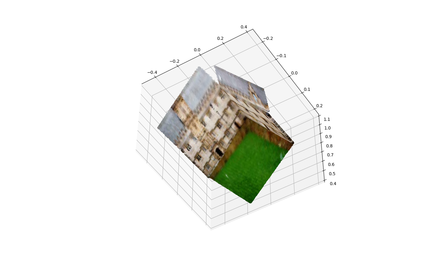
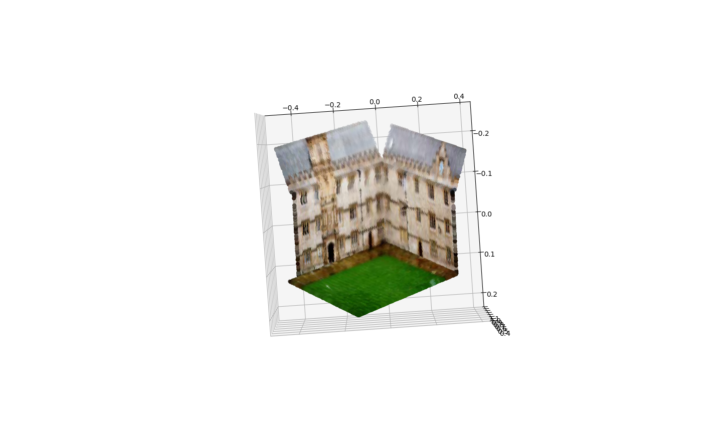
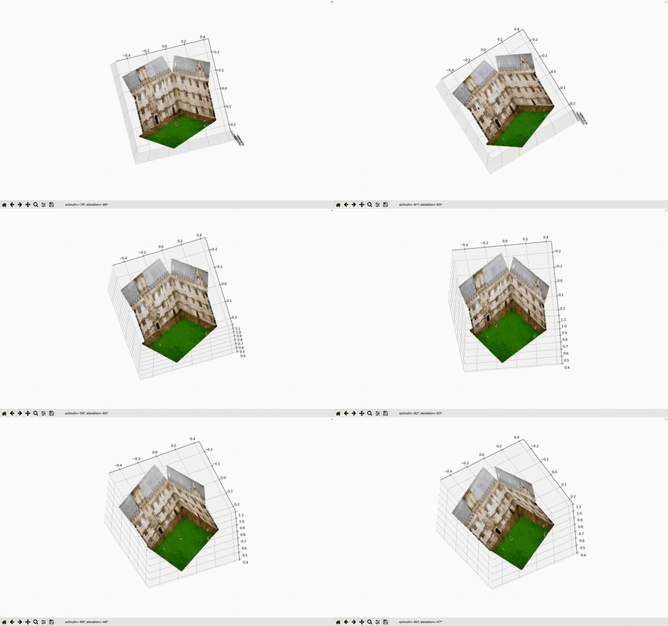
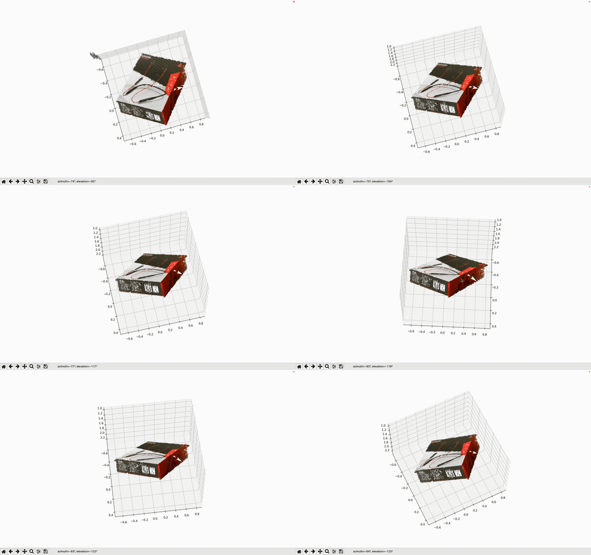
(#) Q3a.
(##) RESULTS
| Input Image | Annotations | Reconstructed view 1 | Reconstructed view 1 |
| ----------- | ----------- | ------- | ------- |
| | | |
(##) BRIEF IMPLEMENTATION DETAILS
1. First using the implementation in Q2a find the intrinsic matrix K
2. Use the plane boundary annotations and K calculated in previous step to compute the plane normals
3. Normals can be computed by using the equation n = $d_{1}$ x $d_{2}$
where $d_{1}$ = $K^{-1}$ $v_{1}$
$d_{2}$ = $K^{-1}$ $v_{2}$
4. Choose a reference point, in this case I chose pixel coordinate (519,245) which is common to 4 different planes
5. Compute the equation of plane using
$n^{T}$ X + a = 0
a = -$n^{T}$($\alpha$ $K^{-1}$ $x_{1}$)
Set the depth of this reference point to 1 unit in 3D world coordinate
6. Now use the annotations provided for each plane to create a mask and then extract all the points which lie in a particular plane, along with their color information.
7. We then compute the distance of the point in 3D from the camera center using the plane equation above. Since we know a, n and K, we use the formula above to compute $\alpha$
8. The alphas calulated in the previous step is multiplied by direction of all the pixels in the plane to compute the ray plane intersection
9. Similarly we also store the color information and finally draw a scatter plot for all the points.
(#) Q3b.
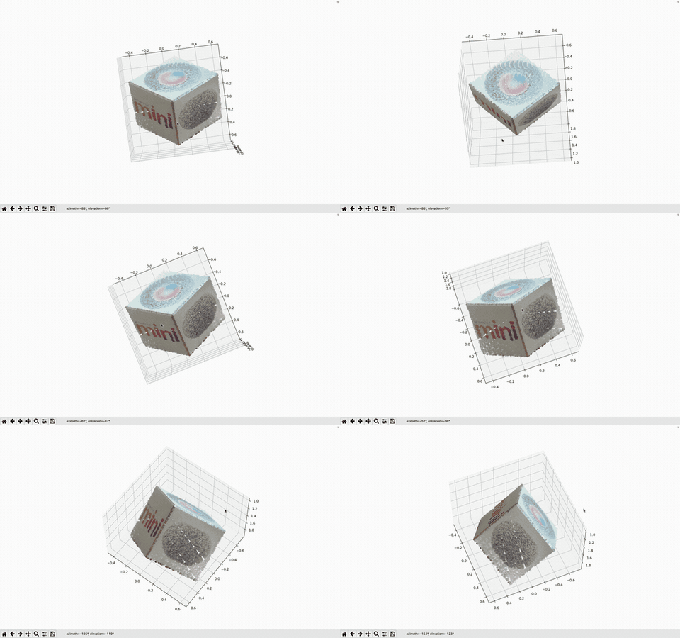
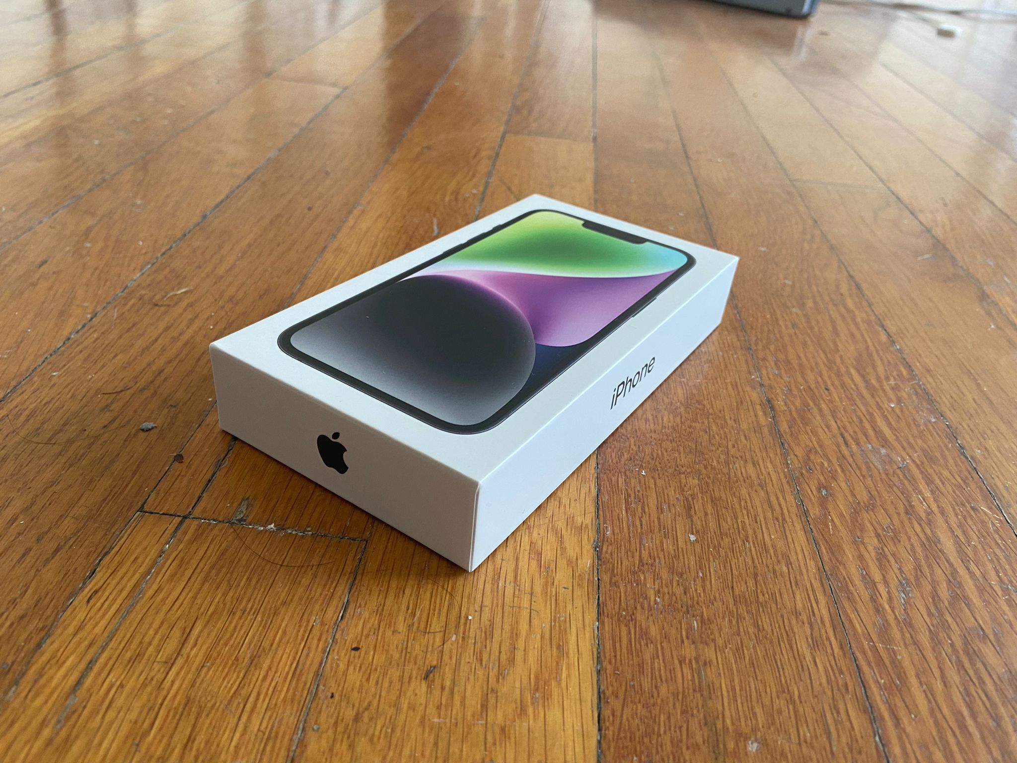
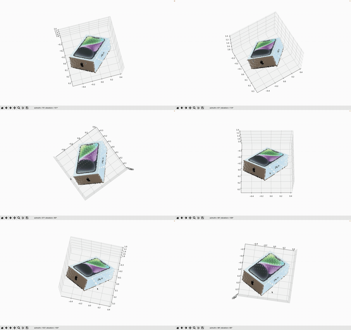
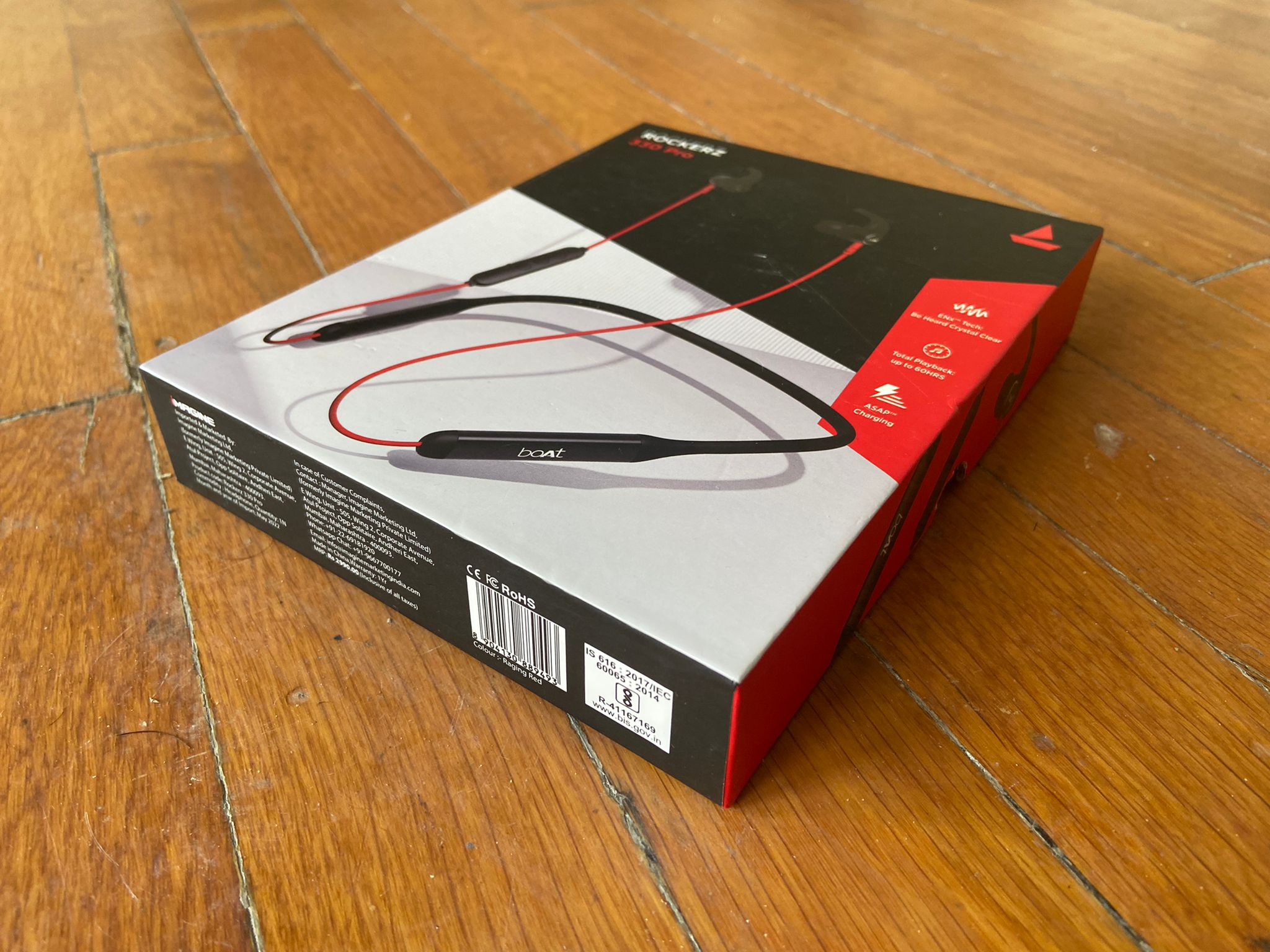
(##) RESULTS
| Input Image | Reconstructed object|
| ----------- | ----------- | ------- |
| | |
| | |
| | |
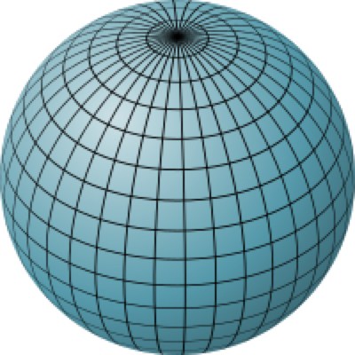 (#) **DEPENDENCY INSTALLATION**
(##) Install conda environment by running
`conda create --name geometry-based-methods`
(##) To install packages
`conda install -r requirements.txt`
(#) **DEPENDENCY INSTALLATION**
(##) Install conda environment by running
`conda create --name geometry-based-methods`
(##) To install packages
`conda install -r requirements.txt`
 (#) Q1b.
(##) RESULTS
Camera Projection Matrix P =
[[ 8.00714922e+00 -3.07780813e+00 1.09825917e+01 9.32661152e+02]
(#) Q1b.
(##) RESULTS
Camera Projection Matrix P =
[[ 8.00714922e+00 -3.07780813e+00 1.09825917e+01 9.32661152e+02] |
|  |
|  |
(#) Q2a.
(##) RESULTS
| Input Image | Annotated Parallel Lines | Vanishing points and principal point |
| ----------- | ----------- | ----------- |
|
|
(#) Q2a.
(##) RESULTS
| Input Image | Annotated Parallel Lines | Vanishing points and principal point |
| ----------- | ----------- | ----------- |
|  |
|  |
|  |
(##) BRIEF IMPLEMENTATION DETAILS
1. Draw 3 sets of parallel lines which are orthogonal to each other or use use the annotations provided.
2. Compute the vanishing points of these lines by taking the cross product between parallel lines
3. Compute the vanishing line by taking cross product between 2 vanishing points. Since we have 3 vanishing points, we can create 3 vanishing lines which all form a triangle.
4. The prinicpal point can then be found out by computing the orthocenter of the triangle
5. Since the pixels are square, we can compute the focal length by applying simple geometric formulae.
6. Intrinsic matrix K obtained by this process is reported below
K= $\begin{bmatrix}
1.15357143e+03 & 0 & 574 \\
0 & 1.15357143e+03 & 431 \\
0 & 0 & 1
\end{bmatrix}$
7. Principal point is (574, 431)
(#) Q2b.
(##) RESULTS
| Input Image | Annotated Square 1 | Annotated Square 2 | Annotated Square 3 |
| ----------- | ----------- | ----------- | ----------- | ----- |
|
|
(##) BRIEF IMPLEMENTATION DETAILS
1. Draw 3 sets of parallel lines which are orthogonal to each other or use use the annotations provided.
2. Compute the vanishing points of these lines by taking the cross product between parallel lines
3. Compute the vanishing line by taking cross product between 2 vanishing points. Since we have 3 vanishing points, we can create 3 vanishing lines which all form a triangle.
4. The prinicpal point can then be found out by computing the orthocenter of the triangle
5. Since the pixels are square, we can compute the focal length by applying simple geometric formulae.
6. Intrinsic matrix K obtained by this process is reported below
K= $\begin{bmatrix}
1.15357143e+03 & 0 & 574 \\
0 & 1.15357143e+03 & 431 \\
0 & 0 & 1
\end{bmatrix}$
7. Principal point is (574, 431)
(#) Q2b.
(##) RESULTS
| Input Image | Annotated Square 1 | Annotated Square 2 | Annotated Square 3 |
| ----------- | ----------- | ----------- | ----------- | ----- |
|  |
|  |
|  |
|  |
| Angle Between planes |
| ----------- | ------|
|Plane 1 and 2: 67.47032019654877|
|Plane 2 and 3: 94.80530541410337|
|Plane 1 and 3: 92.22151037775696|
Intrinsic Matrix:
K= $\begin{bmatrix}
1.08400790e+03 & -1.13937390e+01 & 5.15917724e+02 \\
0 & 1.07775639e+03 & 3.95113033e+02 \\
0 & 0 & 1
\end{bmatrix}$
(##) BRIEF IMPLEMENTATION DETAILS
1. For this question, first compute the homography between the metrically rectified space and image space.
We can use the constraints,
${h_{1}}^T$ $\omega$ $h_{2}$ = 0
${h_{1}}^T$ $\omega$ $h_{1}$ = ${h_{2}}^T$ $\omega$ $h_{2}$
2. Each square will give us two constraints and we will finally have an A matrix which will be 6x6 and we have 6 unknowns in the $\omega$ matrix
3. We can then use SVD to get the 6 values of the $\omega$ matrix
4. Use cholesky decomposition to get K.
5. To compute the angle between the planes, first find normals to the plane. This can be done by first computing the vanshing points and then we can compute the direction of the ray by using
$d_{1}$ = $K^{-1}$ $v_{1}$
$d_{2}$ = $K^{-1}$ $v_{2}$
6. We then compute the cross product between the directions to get the normal to the planes
7. After this take the dot product between the plane normals to get the angles between the planes
(#) Q2c.
(##) RESULTS
| Input Image | Annotations|
| ----------- | ----------- | ------- |
|
|
| Angle Between planes |
| ----------- | ------|
|Plane 1 and 2: 67.47032019654877|
|Plane 2 and 3: 94.80530541410337|
|Plane 1 and 3: 92.22151037775696|
Intrinsic Matrix:
K= $\begin{bmatrix}
1.08400790e+03 & -1.13937390e+01 & 5.15917724e+02 \\
0 & 1.07775639e+03 & 3.95113033e+02 \\
0 & 0 & 1
\end{bmatrix}$
(##) BRIEF IMPLEMENTATION DETAILS
1. For this question, first compute the homography between the metrically rectified space and image space.
We can use the constraints,
${h_{1}}^T$ $\omega$ $h_{2}$ = 0
${h_{1}}^T$ $\omega$ $h_{1}$ = ${h_{2}}^T$ $\omega$ $h_{2}$
2. Each square will give us two constraints and we will finally have an A matrix which will be 6x6 and we have 6 unknowns in the $\omega$ matrix
3. We can then use SVD to get the 6 values of the $\omega$ matrix
4. Use cholesky decomposition to get K.
5. To compute the angle between the planes, first find normals to the plane. This can be done by first computing the vanshing points and then we can compute the direction of the ray by using
$d_{1}$ = $K^{-1}$ $v_{1}$
$d_{2}$ = $K^{-1}$ $v_{2}$
6. We then compute the cross product between the directions to get the normal to the planes
7. After this take the dot product between the plane normals to get the angles between the planes
(#) Q2c.
(##) RESULTS
| Input Image | Annotations|
| ----------- | ----------- | ------- |
| 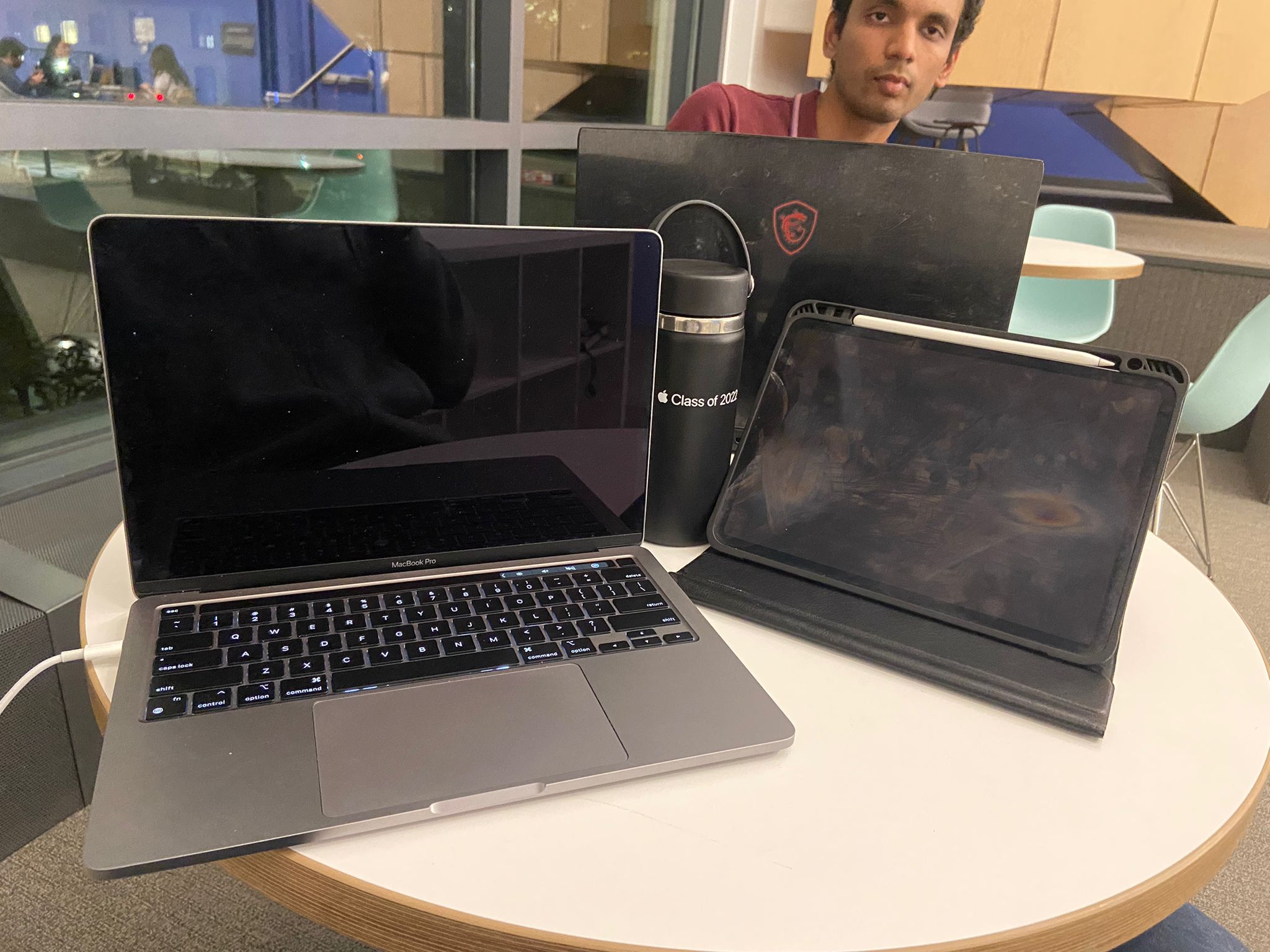 |
| 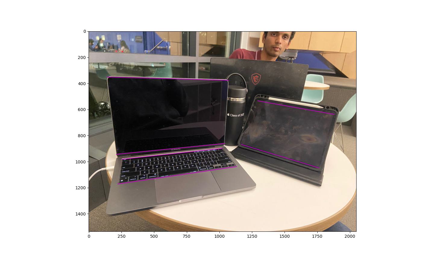 |
| Angle Between planes |
| ----------- | ------|
|Plane 1 and 2: 62.67616513786972|
|Plane 2 and 3: 59.59931039190723|
|Plane 1 and 3: 92.6447856315416|
Intrinsic Matrix:
K= $\begin{bmatrix}
1.66636154e+03 & -7.86141939e+01 & 9.97116245e+02 \\
0 & 1.15357143e+03 & 5.11778464e+02 \\
0 & 0 & 1
\end{bmatrix}$
(##) BRIEF IMPLEMENTATION DETAILS
The implementation is same as the previous question except for the the coordinates in metrically rectified space. Instead of using a square we use the dimensions of the real object
The ratios of the rectangle sides are used to compute K in this case as opposed to using the sides of square
(#) Q3a.
(##) RESULTS
| Input Image | Annotations | Reconstructed view 1 | Reconstructed view 1 |
| ----------- | ----------- | ------- | ------- |
|
|
| Angle Between planes |
| ----------- | ------|
|Plane 1 and 2: 62.67616513786972|
|Plane 2 and 3: 59.59931039190723|
|Plane 1 and 3: 92.6447856315416|
Intrinsic Matrix:
K= $\begin{bmatrix}
1.66636154e+03 & -7.86141939e+01 & 9.97116245e+02 \\
0 & 1.15357143e+03 & 5.11778464e+02 \\
0 & 0 & 1
\end{bmatrix}$
(##) BRIEF IMPLEMENTATION DETAILS
The implementation is same as the previous question except for the the coordinates in metrically rectified space. Instead of using a square we use the dimensions of the real object
The ratios of the rectangle sides are used to compute K in this case as opposed to using the sides of square
(#) Q3a.
(##) RESULTS
| Input Image | Annotations | Reconstructed view 1 | Reconstructed view 1 |
| ----------- | ----------- | ------- | ------- |
| 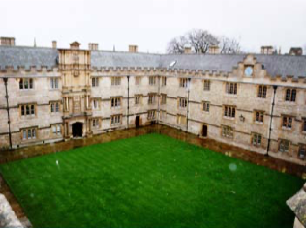 |
| 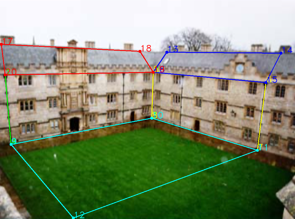 |
|  |
| 
 (##) BRIEF IMPLEMENTATION DETAILS
1. First using the implementation in Q2a find the intrinsic matrix K
2. Use the plane boundary annotations and K calculated in previous step to compute the plane normals
3. Normals can be computed by using the equation n = $d_{1}$ x $d_{2}$
where $d_{1}$ = $K^{-1}$ $v_{1}$
$d_{2}$ = $K^{-1}$ $v_{2}$
4. Choose a reference point, in this case I chose pixel coordinate (519,245) which is common to 4 different planes
5. Compute the equation of plane using
$n^{T}$ X + a = 0
a = -$n^{T}$($\alpha$ $K^{-1}$ $x_{1}$)
Set the depth of this reference point to 1 unit in 3D world coordinate
6. Now use the annotations provided for each plane to create a mask and then extract all the points which lie in a particular plane, along with their color information.
7. We then compute the distance of the point in 3D from the camera center using the plane equation above. Since we know a, n and K, we use the formula above to compute $\alpha$
8. The alphas calulated in the previous step is multiplied by direction of all the pixels in the plane to compute the ray plane intersection
9. Similarly we also store the color information and finally draw a scatter plot for all the points.
(#) Q3b.
(##) RESULTS
| Input Image | Reconstructed object|
| ----------- | ----------- | ------- |
|
(##) BRIEF IMPLEMENTATION DETAILS
1. First using the implementation in Q2a find the intrinsic matrix K
2. Use the plane boundary annotations and K calculated in previous step to compute the plane normals
3. Normals can be computed by using the equation n = $d_{1}$ x $d_{2}$
where $d_{1}$ = $K^{-1}$ $v_{1}$
$d_{2}$ = $K^{-1}$ $v_{2}$
4. Choose a reference point, in this case I chose pixel coordinate (519,245) which is common to 4 different planes
5. Compute the equation of plane using
$n^{T}$ X + a = 0
a = -$n^{T}$($\alpha$ $K^{-1}$ $x_{1}$)
Set the depth of this reference point to 1 unit in 3D world coordinate
6. Now use the annotations provided for each plane to create a mask and then extract all the points which lie in a particular plane, along with their color information.
7. We then compute the distance of the point in 3D from the camera center using the plane equation above. Since we know a, n and K, we use the formula above to compute $\alpha$
8. The alphas calulated in the previous step is multiplied by direction of all the pixels in the plane to compute the ray plane intersection
9. Similarly we also store the color information and finally draw a scatter plot for all the points.
(#) Q3b.
(##) RESULTS
| Input Image | Reconstructed object|
| ----------- | ----------- | ------- |
|  |
|  |
|
|
|  |
|  |
|
|
|  |
|  |
|