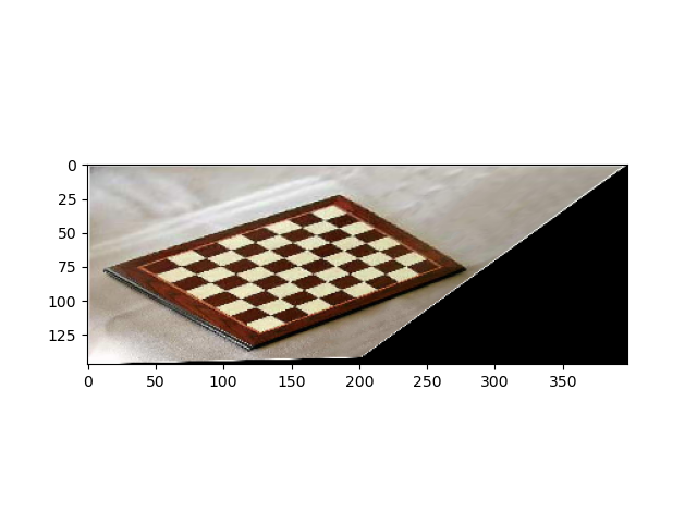
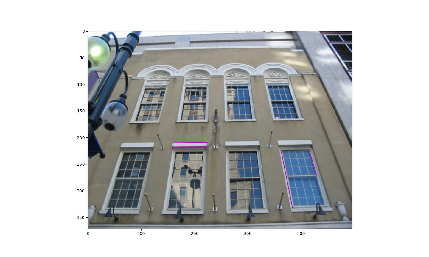
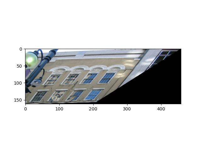
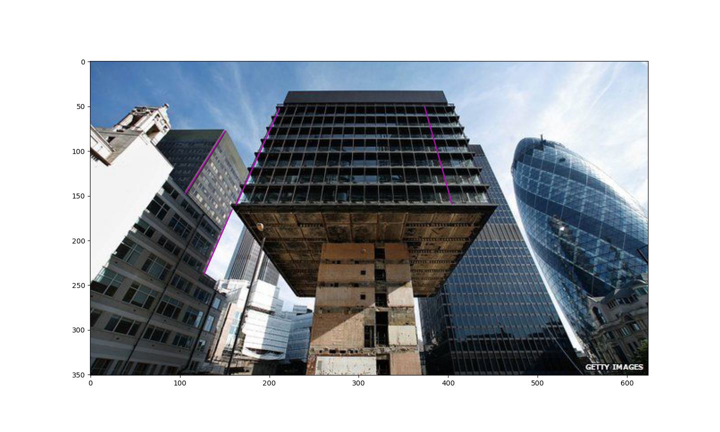
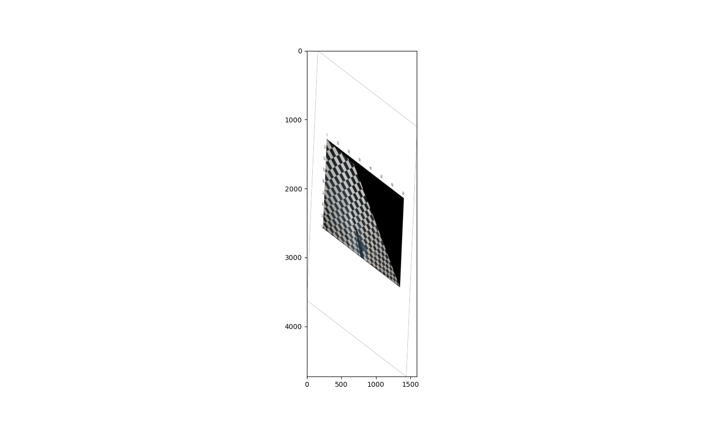
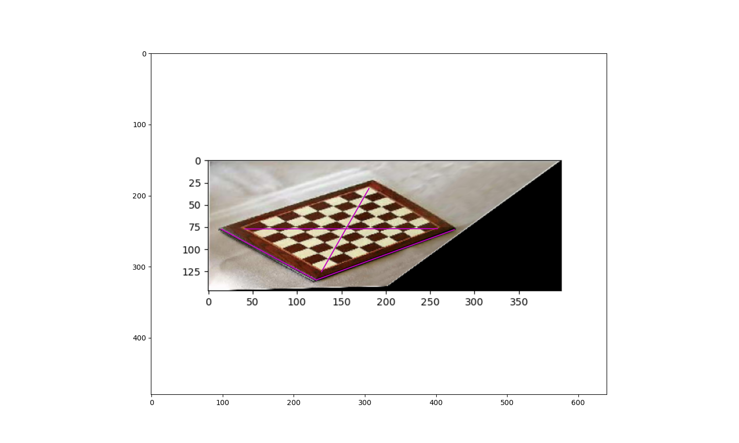
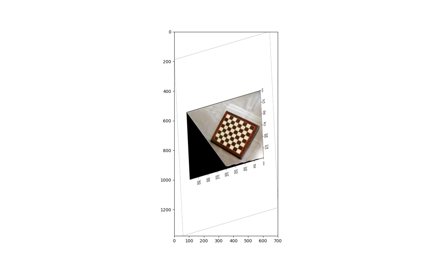
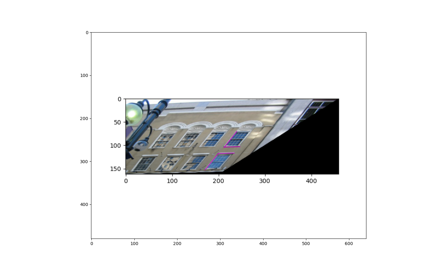
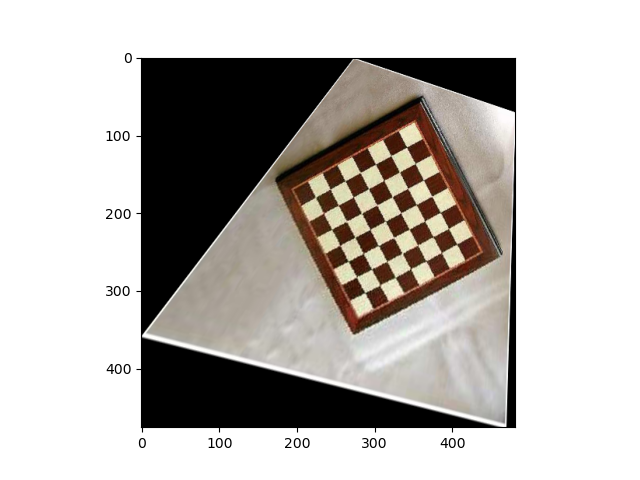
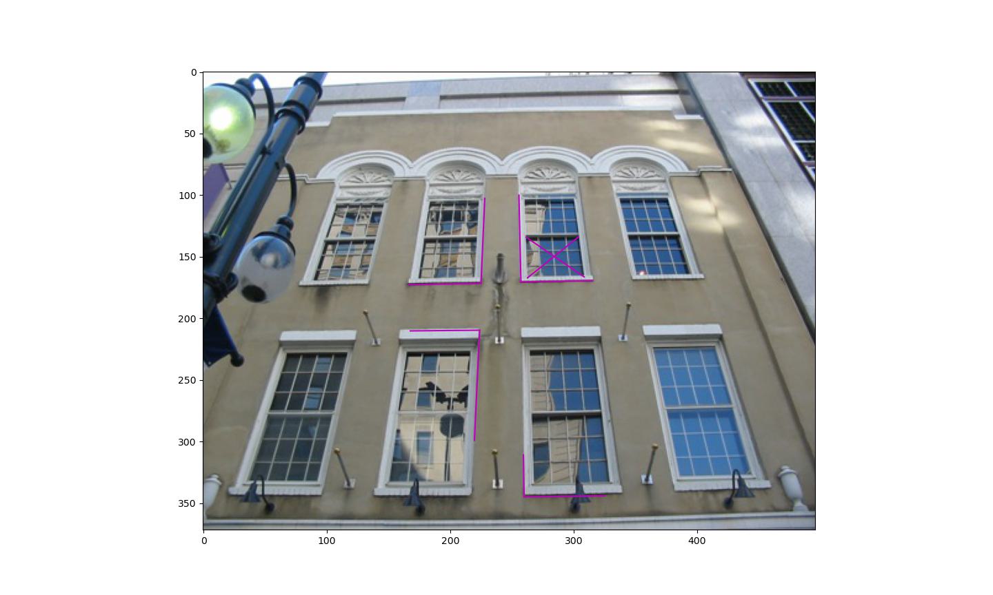
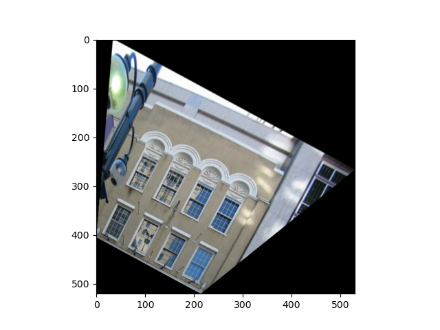
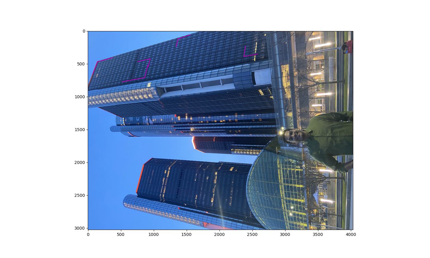
Note: This python is capable of loading images from a folder set by the --data_folder flag. You run the above script and then wait until you mark 8 points (which maybe 2 pair of parallel or 2 pair of perpendicular lines). After annotating 8 points, click on the image anywhere one more time to close the image. You will then be displayed the next image. Repeat the same process. To save the annotated images and correspondences, set the --save_correspondences = True. By default it will save the npz files to a folder called coordinates.
Note: For ease of use, the correspondences have already been saved. Select the appropriate question number, image and coordinate as flags in all of the commands below
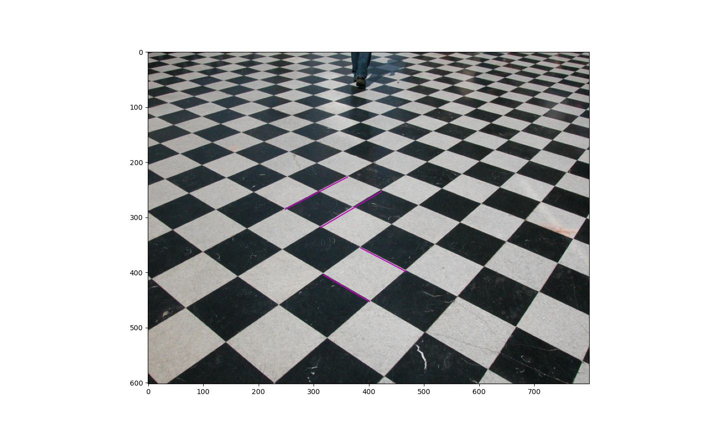
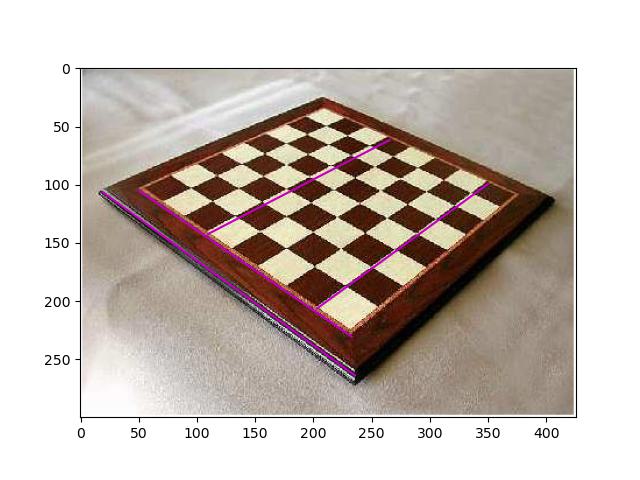
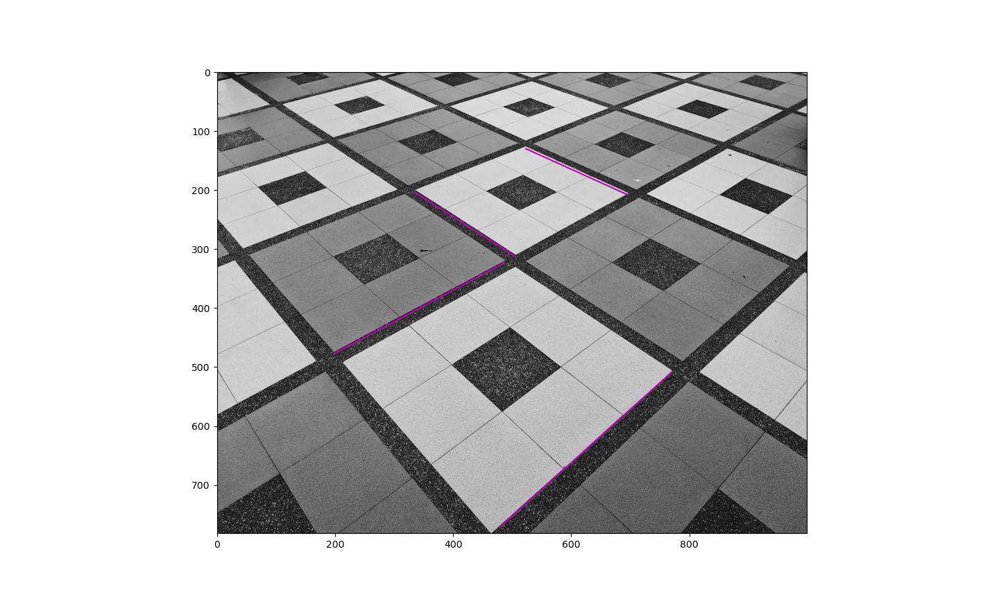
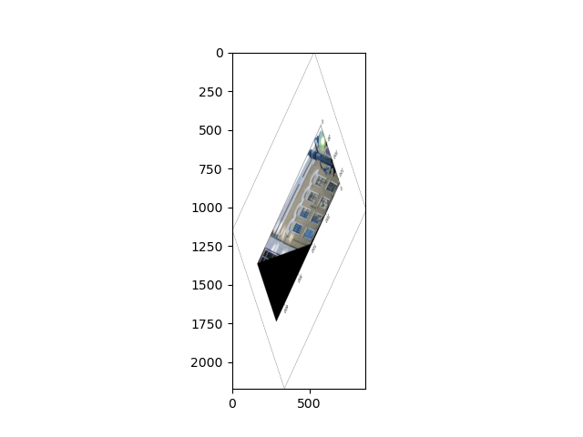
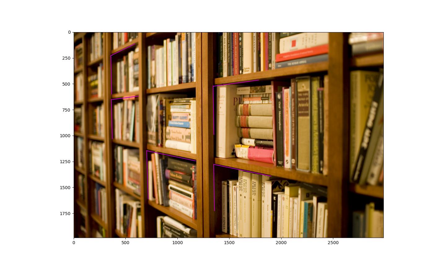
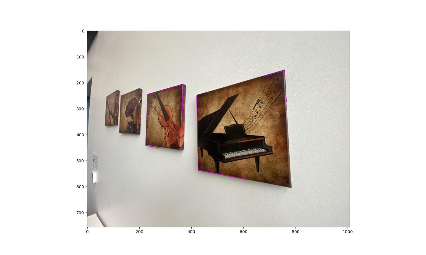
First we mark 8 correspondences using a line picker tool i.e draw 2 sets of parallel lines.
We then use the these coordinates to find out the equation of line joining the two points. This could be found by taking the cross product between the points.
The intersection of two parallel lines gives us a vanishing point and the same can be found by taking the cross product of the two parallel line vectors.
We then find the two vanishing points for 2 sets of parallel lines.
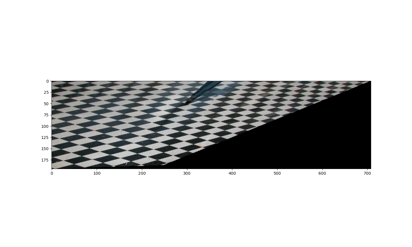
The equation of the line at infinity can then be found by taking the cross product between the two vanishing points.
The resultant vector (line l = [l1,l2,l3]) that we get can then be used to construct the matrix H = ⎣⎡10l101l200l3⎦⎤
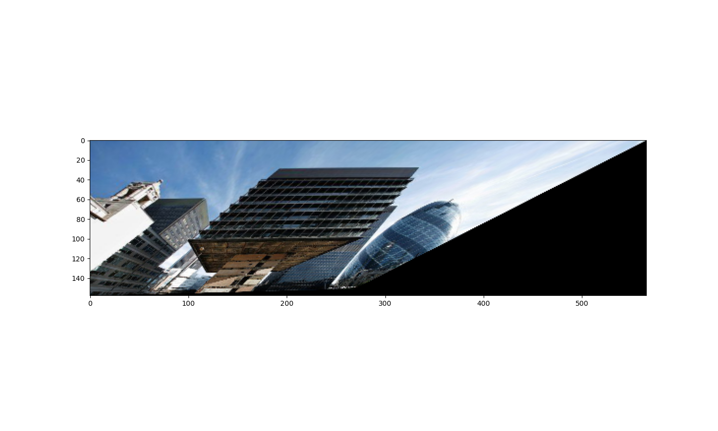
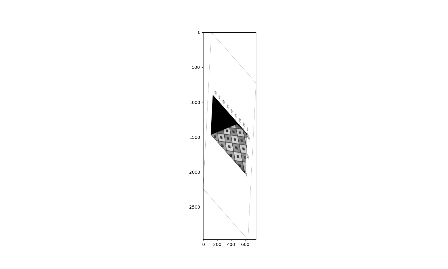
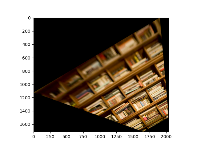
This matrix can then be multiplied with the image to get affine rectification
Q2. METRIC RECTIFICATION
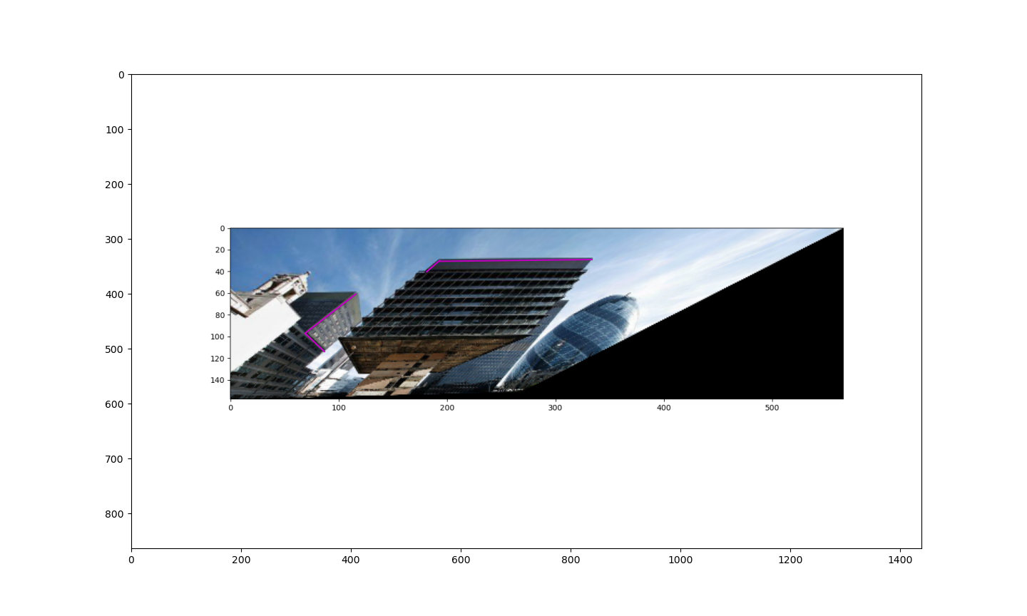
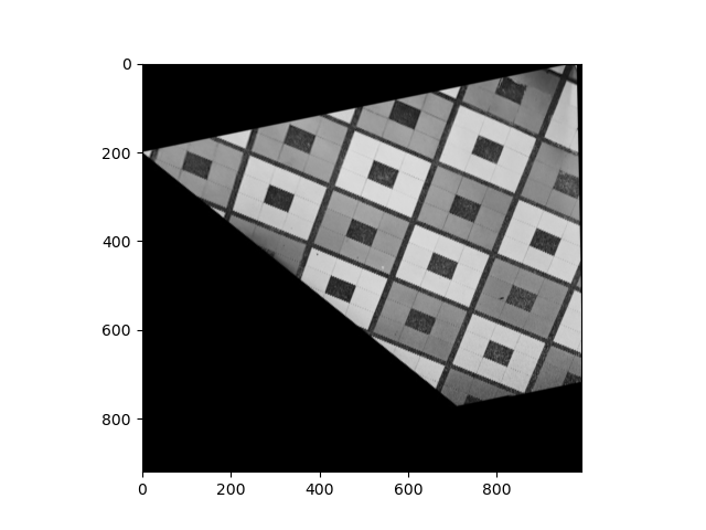
Affine Rectified Image with correspondence
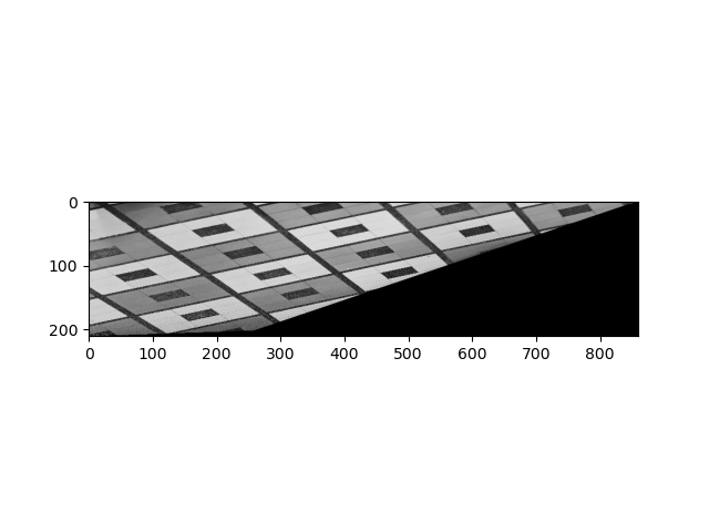
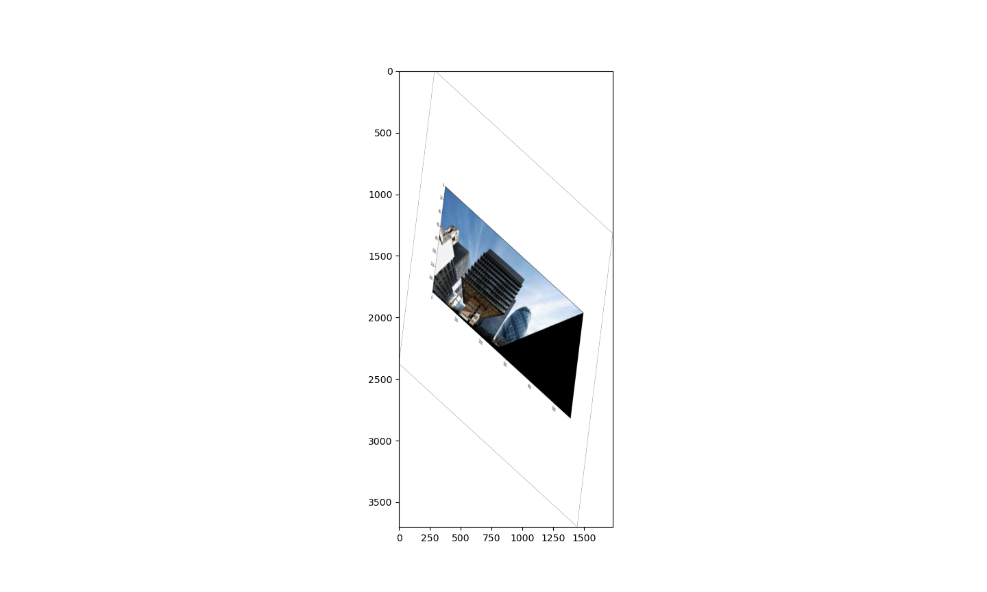
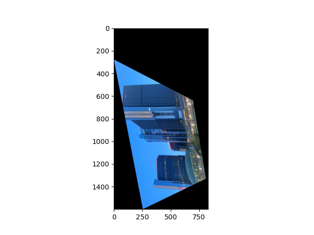
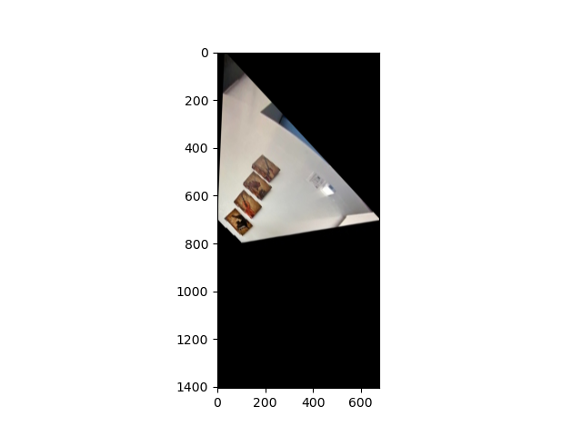
Metric Rectified image
Cosine Before
Cosine After
0.8528
-1.32e-13
0.4881
-1.078e-16
0.6431
0.00002
0.1473
9.6815e-16
0.6759
0.00003
BRIEF DESCRIPTION OF IMPLEMENTATION
First we mark 8 correspondences using a line picker tool i.e draw 2 sets of perpendicular lines on the affine rectfied image.
We then use the these coordinates to find out the equation of line joining the two points. This could be found by taking the cross product between the points.
We then use the equation of line conic lC∞m = 0 .This can be represented as Ac = 0.
where A = ⎣⎡a1[0]∗a2[0]b1[0]∗b2[0]0(a1[0]∗a2[1]+a1[1]∗a2[0])/2(b1[0]∗b2[1]+b1[1]∗b2[0])/20a1[1]∗a2[1]b1[1]∗b2[1]0⎦⎤
We then use SVD to find out the values that help us construct the conic matrix. Note: Since the images are affine rectified first, we have values for only a,b,c and d,e,f =0
We then compute the matrix C∞∗ = ⎣⎡ab/2d/2b/2ce/2d/2e/2f⎦⎤
After this we take the SVD of the above matrix and then construct H matrix as follows:
H = ⎣⎡1/s10001/s20001⎦⎤ * vh
where s1 = σ1
s2 = σ2
This matrix can then be multiplied with the image to get metric rectification
Q3. PLANAR HOMOGRAPHY
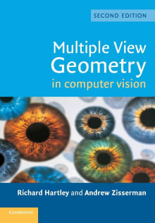
Source Image
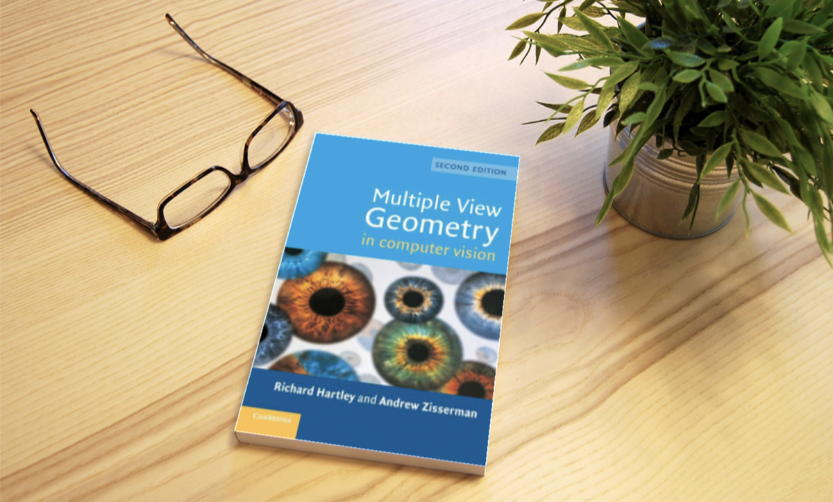
Destination Image
Homography
BRIEF DESCRIPTION OF IMPLEMENTATION
First we mark 4 correspondences in the source image and in the destination image. These points are the corner points of the book.
We then normalize these coordinates such that the points are centered around the mean and the maximum distance from the center is square root of 2.
We then use these normalized co-ordinates to construct the A matrix such that Ah=0
Since the degree of freedom is 8, we need 8 equations to solve for the elements in the homography matrix. Each correspondence gives us 2 constraints. So we need 4 correspondences for 8 equations
We then construct the A matrix as follows
A = [−xd[0]0−yd[0]0−100−xd[0]0−yd[0]0−1xd[0]∗xs[0]xd[0]∗ys[0]yd[0]∗xs[0]yd[0]∗ys[0]xs[0]ys[0]]
where, d : destination image,
s:source image
By solving the above equation Ah=0 using SVD, we obtain the 9 values of homography matrix.
We then denormalize the image to get the cooridnates in the original space.
We then create a mask on the destination image and warp the source image
with our homography matrix
This image is then laid on top of our perspective image (in this case book on a desk)
EXTRA CREDITS
Q4. METRIC RECTIFICATION WITHOUT AFFINE RECTIFICATION
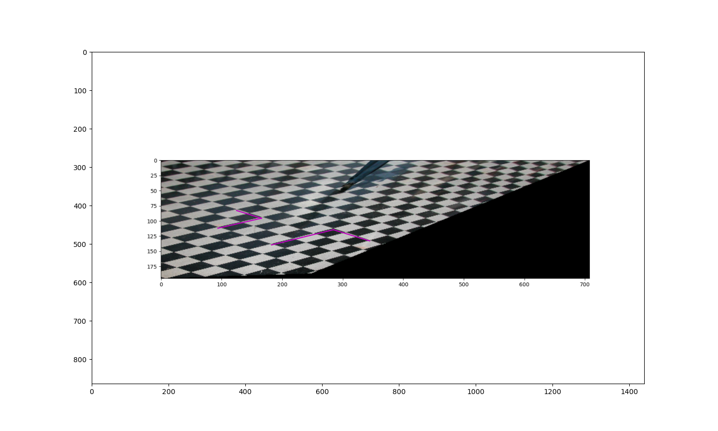
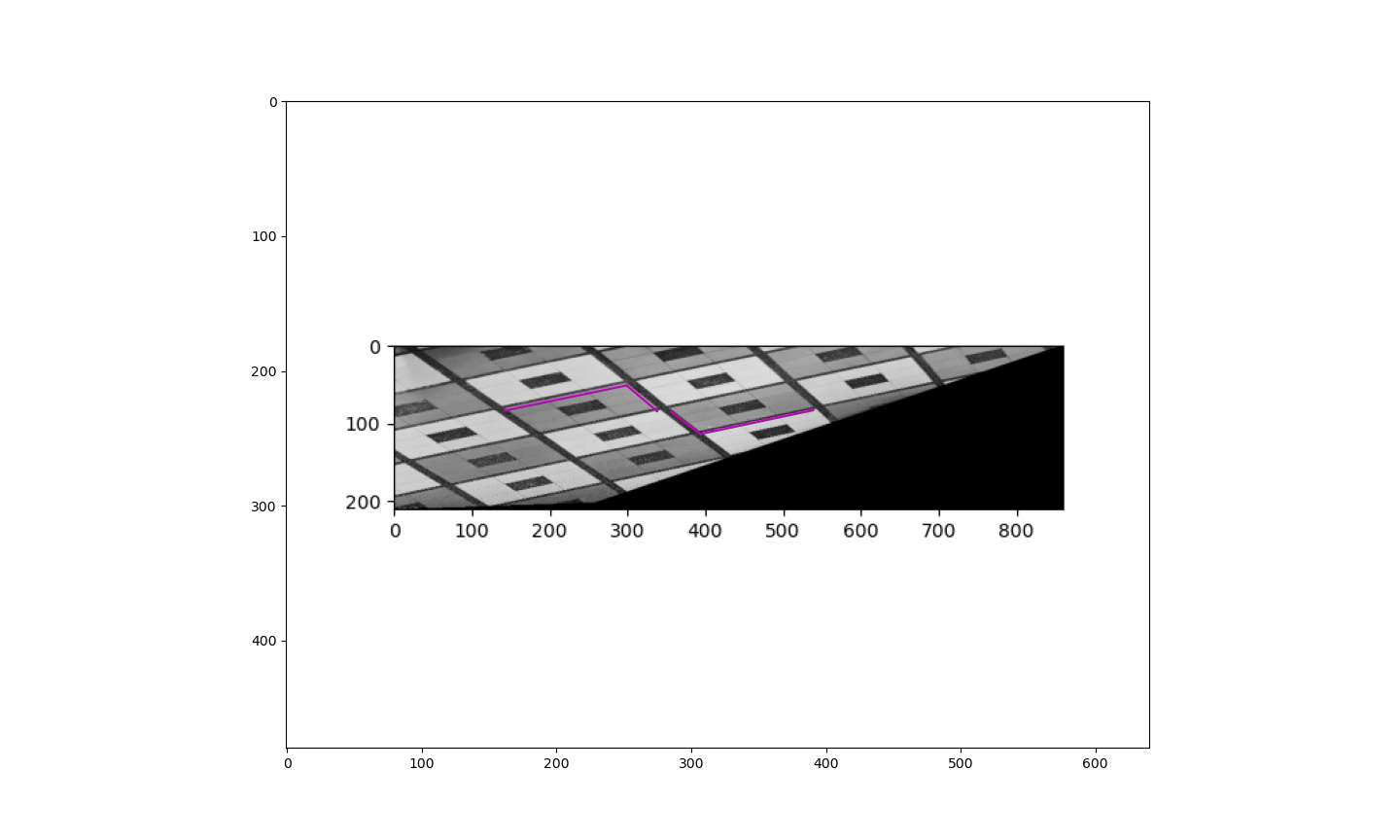
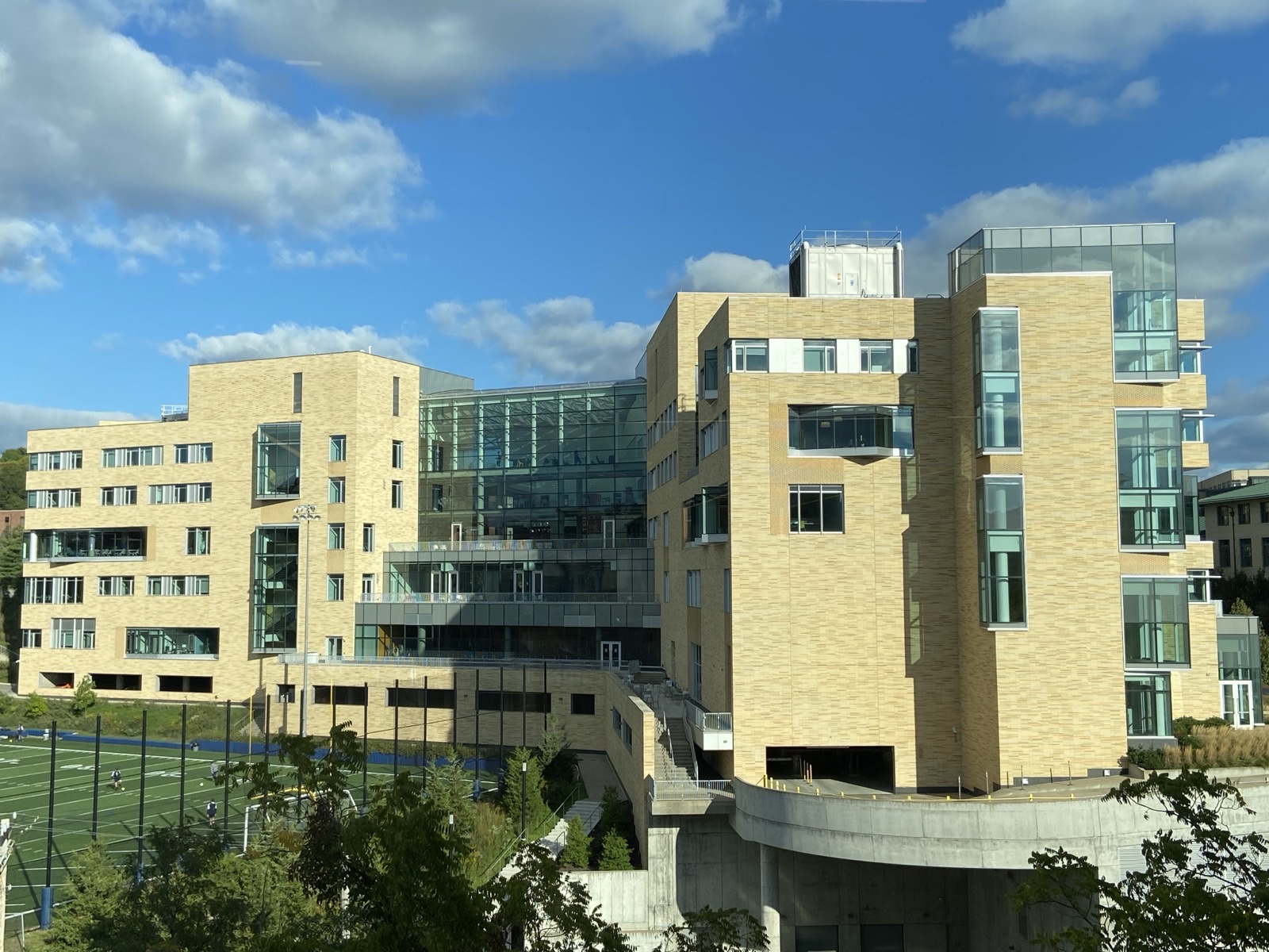
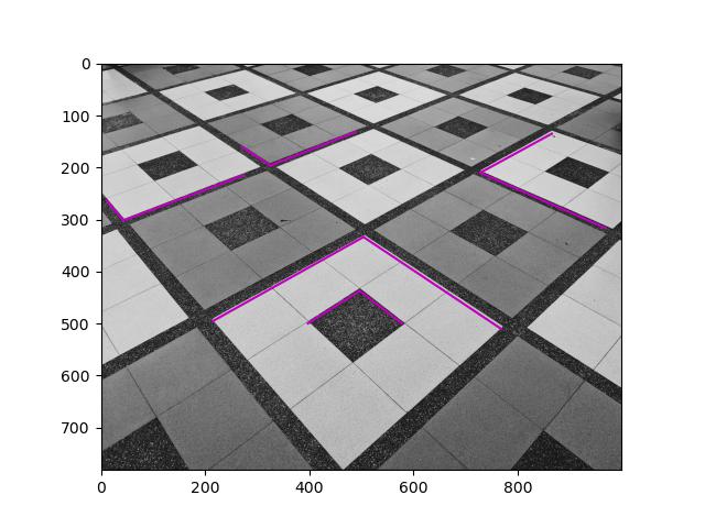
Original Image with correspondence
Metric Rectified image
Cosine Before
Cosine After
0.4234
0.0206
0.8999
3.25e-16
0.7656
0.0032
0.9667
4.089e-16
0.8765
8.385e-16
0.9696
3.41e-14
BRIEF DESCRIPTION OF IMPLEMENTATION
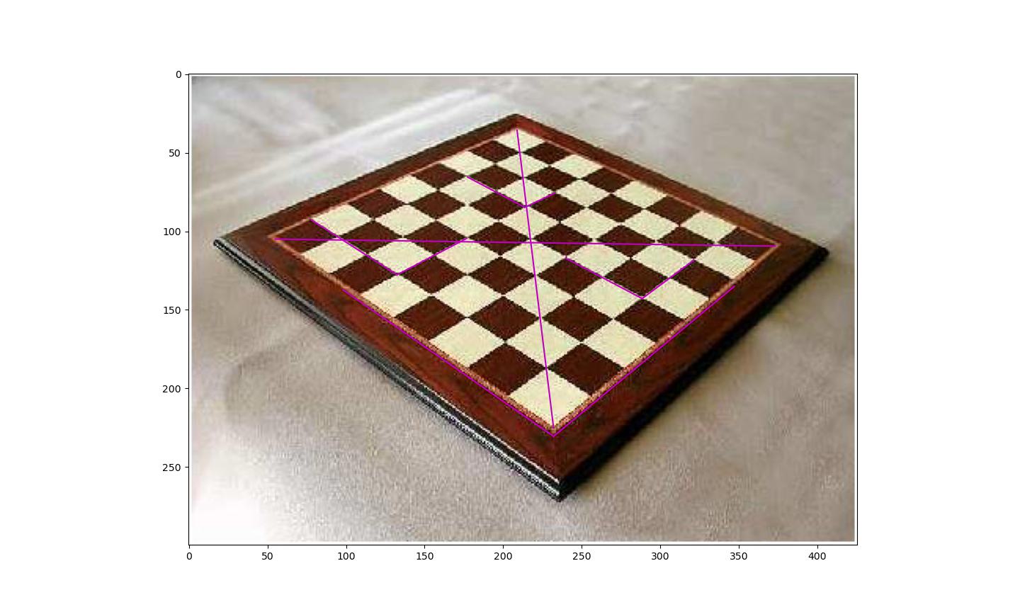
First we mark 20 correspondences using a line picker tool i.e draw 5 sets of perpendicular lines on the original image.
We then use the these coordinates to find out the equation of line joining the two points. This could be found by taking the cross product between the points.
We then use the equation of line conic lC∞m = 0 .This can be represented as Ac = 0.
where A = ⎣⎡a1[0]∗a2[0]b1[0]∗b2[0]c1[0]∗c2[0]d1[0]∗d2[0]e1[0]∗e2[0](a1[0]∗a2[1]+a1[1]∗a2[0])/2(b1[0]∗b2[1]+b1[1]∗b2[0])/2(c1[0]∗c2[1]+c1[1]∗c2[0])/2(d1[0]∗d2[1]+d1[1]∗d2[0])/2(e1[0]∗e2[1]+e1[1]∗e2[0])/2a1[1]∗a2[1]b1[1]∗b2[1]c1[1]∗c2[1]d1[1]∗d2[1]e1[1]∗e2[1](a1[0]∗a2[2]+a1[2]∗a2[0])/2(b1[0]∗b2[2]+b1[2]∗b2[0])/2(c1[0]∗c2[2]+c1[2]∗c2[0])/2(d1[0]∗d2[2]+d1[2]∗d2[0])/2(e1[0]∗e2[2]+e1[2]∗e2[0])/2(a1[1]∗a2[2]+a1[2]∗a2[1])/2(b1[1]∗b2[2]+b1[2]∗b2[1])/2(c1[1]∗c2[2]+c1[2]∗c2[1])/2(d1[1]∗d2[2]+d1[2]∗d2[1])/2(e1[1]∗e2[2]+e1[2]∗e2[1])/2a1[2]∗a2[2]b1[2]∗b2[2]c1[2]∗c2[2]d1[2]∗d2[2]e1[2]∗e2[2]⎦⎤
Here a1,a2; b1,b2; c1,c2; d1,d2; e1,e2 represent 5 pair of perpendicular lines
We then use SVD to find out the values that help us construct the conic matrix. These values are a,b,c,d,e,f
We then compute the matrix C∞∗ = ⎣⎡ab/2d/2b/2ce/2d/2e/2f⎦⎤
After this we take the SVD of the above matrix and then construct H matrix as follows:
H = ⎣⎡1/s10001/s20001⎦⎤ * vh
where s1 = σ1
s2 = σ2
We finally use this matrix and rectify our original image
Q5. PLANAR HOMOGRAPHY WITH MULTIPLE IMAGES
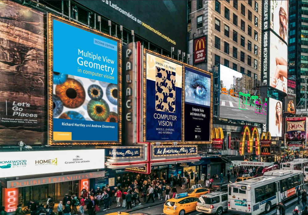
Destination Image
Homography
BRIEF DESCRIPTION OF IMPLEMENTATION
First we mark 4 correspondences in the source image and 4 correspondences in the destination image. These points are the corner points of the timessquare billboard and 4 corners of the image we have captured
We then normalize these coordinates such that the points are centered around the mean and the maximum distance from the center is square root of 2.
We then use these normalized co-ordinates to construct the A matrix such that Ah=0
Since the degree of freedom is 8, we need 8 equations to solve for the elements in the homography matrix. Each correspondence gives us 2 constraints. So we need 4 correspondences for 8 equations
We then construct the A matrix as follows
A = [−xd[0]0−yd[0]0−100−xd[0]0−yd[0]0−1xd[0]∗xs[0]xd[0]∗ys[0]yd[0]∗xs[0]yd[0]∗ys[0]xs[0]ys[0]]
where, d : destination image,
s:source image
By solving the above equation Ah=0 using SVD, we obtain the 9 values of homography matrix.
We then denormalize the image to get the cooridnates in the original space.
We then create a mask on the destination image and warp the source image
with our homography matrix
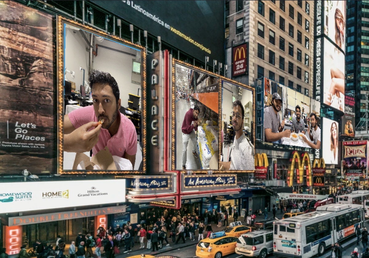
This image is then laid on top of our perspective image (in this case timessquare billboard)
We then use this composite image and use that as the destination image in the next step.
We repeat steps 2-10, until we have all the images we wanted to be replaced in the destination image.